Search Algorithms
Search is one of the most fundamental concepts in artificial intelligence. Before machine learning rose to prominence, AI research treated search as its central problem. Early systems such as Newell and Simon’s General Problem Solver (1957) framed reasoning itself as search: to solve a problem, you define the states you can be in, the actions that move between them, and a goal test, then explore the resulting space until you reach a goal. This idea still drives planning, theorem proving, route finding, and game playing today. In this chapter we explore how to implement classic search algorithms in Scala 3, taking advantage of its elegant functional features and clean syntax.
We will build three examples:
- Graph Search: Implementing Depth-First Search (DFS) and Breadth-First Search (BFS) over a graph of cities.
- Maze Solving: Generating a random maze using depth-first carving and solving it with BFS to guarantee the shortest path.
- Game Tree Search: Implementing the Minimax algorithm with alpha-beta pruning to play an optimal game of Tic-Tac-Toe.
All code is in the directory source-code/search.
Search as a Formal Problem
The three examples in this chapter look different on the surface, but they share one structure. We can state any of them with five parts:
- A state space: the set of all configurations the world can take. For the city to city route planning graph a state is a graph where the nodes are city names, for the maze it is a grid cell, and for Tic-Tac-Toe it is a board position.
- An initial state: where the search begins.
- A successor function: given a state, it returns the states reachable in one step. In our code this is
neighbors,openNeighbors, oremptyCells. - A goal test: a predicate that tells us when we have finished.
- A path cost: a number we may want to minimize, such as the count of edges on the path.
A search algorithm grows two sets as it runs. The frontier holds states we have generated but not yet expanded. The explored set (the visited set in our code) holds states we have already expanded, so we never process one twice. The algorithms in this chapter differ in just one way: how they pick the next state from the frontier. That single choice fixes both their behavior and their cost.
We judge a search algorithm on four properties:
- Completeness: does it always find a solution when one exists?
- Optimality: does it find the lowest-cost solution?
- Time complexity: how many states does it generate?
- Space complexity: how many states does it hold in memory at once?
We write 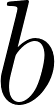 for the branching factor (the average number of successors per state) and
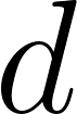 for the depth of the shallowest goal. These two numbers drive the cost of every algorithm below.
Representing Graphs
To search a graph, we first need to represent it. We define a simple immutable representation in search/Graph.scala using Scala 3 case classes. A node contains a name and coordinates, and the graph itself tracks a vector of nodes and undirected edge pairs:
 1 case class Node(name: String, x: Int, y: Int)
 2
 3 case class Graph(nodes: Vector[Node], edges: Vector[(Int, Int)]):
 4
 5   /** Return indices of all nodes directly connected to `node`. */
 6   def neighbors(node: Int): List[Int] =
 7     edges.collect:
 8       case (a, b) if a == node => b
 9       case (a, b) if b == node => a
10     .toList
11
12   /** Euclidean distance between two nodes (for A* or display). */
13   def distance(a: Int, b: Int): Double =
14     val dx = nodes(a).x - nodes(b).x
15     val dy = nodes(a).y - nodes(b).y
16     math.sqrt(dx * dx + dy * dy)
17
18 object Graph:
19   /** Build a graph from a list of (name, x, y) and edge pairs (name, name). */
20   def apply(nodeDefs: List[(String, Int, Int)], edgeDefs: List[(String, String)]): Graph =
21     val nodes = nodeDefs.map((n, x, y) => Node(n, x, y)).toVector
22     val nameToIndex = nodes.zipWithIndex.map((n, i) => n.name -> i).toMap
23     val edges = edgeDefs.map((a, b) => (nameToIndex(a), nameToIndex(b))).toVector
24     Graph(nodes, edges)
This is an edge list representation. We store nodes in a Vector, which gives effectively constant-time indexed access, and we refer to each node by its integer index rather than by name. Integer indices are cheap to compare, cheap to store in a Set, and let us key the visited set on a primitive rather than on a string.
The neighbors method scans the whole edge list on each call, so it costs 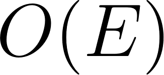 time for
 edges. For the small graphs in this chapter that cost does not matter. For a large graph you would instead precompute an adjacency list, a
Map[Int, List[Int]] that answers neighbors in O(1) time at the cost of 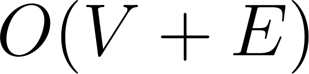 memory. The edge list keeps the example short and makes the undirected nature of the graph explicit: a single pair
(a, b) yields b as a neighbor of a and a as a neighbor of b, which is exactly what the two case clauses in the collect express.
We also include a distance method that returns the straight-line (Euclidean) distance between two nodes. Uninformed searches like DFS and BFS ignore it, but an informed search such as A* would use it as a heuristic: an estimate of the remaining cost to the goal that guides the search toward promising nodes first.
Depth-First and Breadth-First Graph Search
DFS and BFS are the two basic uninformed (or “blind”) search strategies. Neither uses any knowledge of where the goal lies, so both differ only in the order they pull states off the frontier. DFS treats the frontier as a stack and always expands the deepest unexpanded state. BFS treats the frontier as a queue and always expands the shallowest. That one difference produces sharply different guarantees:
| Property | DFS | BFS |
|---|---|---|
| Complete on a finite graph | Yes | Yes |
| Optimal (fewest edges) | No | Yes |
Time (tree with branching b, solution depth d) |
O(b^m) |
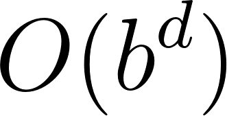
O(b^d) |
| Space | O(b, m) |
O(b^d) |
Here 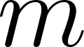 is the maximum depth of the state space, which can be much larger than (the depth searched before finding the goal node). The table shows the core trade-off. BFS keeps a whole layer of the frontier in memory, so its space cost grows exponentially with depth, but it never overlooks a shallow goal. DFS holds only the current path plus its siblings, so its memory cost is linear, but it can plunge down a deep or infinite branch and miss a nearby solution.
Both of our implementations track a visited set. On a general graph with cycles this set is what keeps the searches complete: without it, DFS could loop forever around a cycle. Tracking visited states bounds both searches at time and 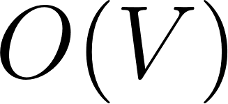 space, since each node is expanded at most once and each edge examined at most twice. We trade memory for the guarantee that we never revisit a state.
We implement both searches in a purely functional manner in search/GraphSearch.scala. Each returns an Option[List[Int]] holding the path of node indices from start to goal, or None if no path exists.
DFS uses recursive backtracking. It explores as deep as possible along each branch before backing up, and it carries the visited set forward so it never re-enters a node already on the current search:
 1   /** Depth-first search using recursive backtracking. */
 2   def depthFirst(graph: Graph, start: Int, goal: Int): Option[List[Int]] =
 3     def search(node: Int, visited: Set[Int]): Option[List[Int]] =
 4       if node == goal then Some(List(goal))
 5       else
 6         val nextNodes = graph.neighbors(node).filterNot(visited.contains)
 7         nextNodes.view
 8           .flatMap(n => search(n, visited + n))
 9           .headOption
10           .map(node :: _)
11
12     search(start, Set(start))
The recursion carries the base case cleanly: if node is the goal, we return a one-element path. Otherwise we filter out visited neighbors and search each in turn. The key detail is .view. It turns the flatMap into a lazy computation, so headOption forces only as many recursive searches as it needs to find the first branch that reaches the goal. The moment one branch succeeds, the remaining neighbors are never explored. This is the functional equivalent of an early return inside a loop, and it keeps DFS from doing needless work after it finds a path. Each successful frame then prepends its own node with node :: _, so the path is rebuilt in the correct start-to-goal order as the recursion unwinds.
Breadth First Search (BFS) explores all neighbors at the current depth before moving deeper. We implement it with a queue of partial paths. Because it always expands the shallowest node first, the first time it reaches the goal it has done so by a path with the fewest possible edges. This is why BFS is optimal for unweighted graphs: every path of length 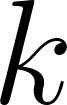 is fully explored before any path of length
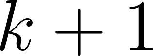 begins, so no shorter path to the goal can remain undiscovered:
 1   /** Breadth-first search using a queue of partial paths.
 2     * Always finds the shortest path (fewest edges).
 3     */
 4   def breadthFirst(graph: Graph, start: Int, goal: Int): Option[List[Int]] =
 5     import scala.collection.immutable.Queue
 6
 7     @annotation.tailrec
 8     def search(queue: Queue[(Int, List[Int])], visited: Set[Int]): Option[List[Int]] =
 9       if queue.isEmpty then None
10       else
11         val ((node, path), rest) = queue.dequeue
12         if node == goal then Some(path.reverse)
13         else
14           val nextNodes = graph.neighbors(node).filterNot(visited.contains)
15           val newVisited = visited ++ nextNodes
16           val newEntries = nextNodes.map(n => (n, n :: path))
17           search(rest.enqueueAll(newEntries), newVisited)
18
19     search(Queue((start, List(start))), Set(start))
Two implementation choices deserve attention. First, the @annotation.tailrec annotation asks the compiler to verify that search is tail recursive. Because the recursive call is the last action in the function, the compiler rewrites it into a plain loop, so BFS runs in constant stack space no matter how large the graph. Second, we add nodes to the visited set the moment we enqueue them (newVisited = visited ++ nextNodes), not when we later dequeue them. This matters: if two different frontier nodes both border the same unvisited node, marking on enqueue stops that node from entering the queue twice. Without it the queue could hold many copies of the same state, which wastes memory and can break the shortest-path reasoning. We build each partial path by prepending (n :: path), which is a constant-time operation on an immutable list, then reverse once at the end when we return the finished path.
We run all the search examples with one test program. Here we only show the output for the Depth First Search (DFS) and Breadth First Search (BFS) city route planing example:
1  $ scala-cli run .
2 Starting compilation server
3 ==================================================
4 Graph Search Demo
5 ==================================================
6
7 Searching from Atlanta to Erie:
8   DFS path: Atlanta → Baltimore → Chicago → Erie
9   BFS path: Atlanta → Chicago → Erie
Maze Generation and Solving
Solving mazes is another classic search benchmark. We represent a maze as a 2D grid of booleans where true is a wall and false is an open passage. We generate a random maze using a DFS-based recursive backtracking algorithm (carving paths through walls) in search/Maze.scala:
 1 case class Location(row: Int, col: Int)
 2
 3 case class Maze(grid: Vector[Vector[Boolean]], rows: Int, cols: Int):
 4   def isBlocked(loc: Location): Boolean =
 5     loc.row < 0 || loc.row >= rows ||
 6     loc.col < 0 || loc.col >= cols ||
 7     grid(loc.row)(loc.col)
 8
 9   def openNeighbors(loc: Location): List[Location] =
10     List(
11       Location(loc.row - 1, loc.col),
12       Location(loc.row + 1, loc.col),
13       Location(loc.row, loc.col - 1),
14       Location(loc.row, loc.col + 1)
15     ).filterNot(isBlocked)
The generator is worth understanding, because it explains why BFS behaves the way it does on the result. The recursive backtracker starts with every cell walled off, then carves a path. It marks the current cell open, shuffles the four directions, and for each direction steps two cells away. If that far cell is still a wall (still unvisited), it knocks out the wall between the two cells and recurses into the far cell.
Notice in the first block that DFS and BFS return different paths from Atlanta to Erie: DFS follows the first branch it happens to descend (through Denver and Chicago), while BFS finds the shorter two-edge route through Chicago, exactly as the optimality guarantee predicts:
 1 object Maze:
 2   /** Generate a random maze using recursive backtracking (DFS carving). */
 3   def generate(rows: Int, cols: Int, seed: Long = 42L): Maze =
 4     val rng = scala.util.Random(seed)
 5     val grid = Array.fill(rows, cols)(true) // start all walls
 6
 7     def carve(r: Int, c: Int): Unit =
 8       grid(r)(c) = false
 9       val directions = rng.shuffle(List((0, 2), (0, -2), (2, 0), (-2, 0)))
10       for (dr, dc) <- directions do
11         val nr = r + dr
12         val nc = c + dc
13         if nr >= 0 && nr < rows && nc >= 0 && nc < cols && grid(nr)(nc) then
14           grid(r + dr / 2)(c + dc / 2) = false // knock out wall between
15           carve(nr, nc)
16
17     carve(1, 1)
18     Maze(grid.map(_.toVector).toVector, rows, cols)
Cells sit on odd coordinates and the wall between two cells sits at the midpoint, which is why the steps are of size two and the wall is knocked out at r + dr / 2. Because the algorithm only ever carves into a cell that no path has reached yet, it can never create a loop, and because it visits every reachable cell, it leaves no region walled off. The result is a perfect maze: a spanning tree over the grid of cells with exactly one simple path between any two cells and no cycles.
That property has a direct consequence for solving. On a perfect maze the path between start and goal is unique, so any complete search finds it. BFS still earns its keep, because the moment you add loops (a “braided” maze with more than one route) BFS returns the shortest route while DFS returns the first one it stumbles into, which may wander. We solve the maze with either MazeSearch.depthFirst or MazeSearch.breadthFirst. The BFS solver uses the exact same queue-based strategy shown for graphs, so it carries the same shortest-path guarantee:
 1   /** Solve a maze using breadth-first search (shortest path). */
 2   def breadthFirst(maze: Maze, start: Location, goal: Location): Option[List[Location]] =
 3     import scala.collection.immutable.Queue
 4
 5     @annotation.tailrec
 6     def search(queue: Queue[(Location, List[Location])], visited: Set[Location]): Option[List[Location]] =
 7       if queue.isEmpty then None
 8       else
 9         val ((loc, path), rest) = queue.dequeue
10         if loc == goal then Some(path.reverse)
11         else
12           val nextLocs = maze.openNeighbors(loc).filterNot(visited.contains)
13           val newVisited = visited ++ nextLocs
14           val newEntries = nextLocs.map(n => (n, n :: path))
15           search(rest.enqueueAll(newEntries), newVisited)
16
17     search(Queue((start, List(start))), Set(start))
The only change from the graph version is that the state is a Location (a row and column) instead of an integer index, and the successor function is openNeighbors instead of neighbors. The maze is a graph whose nodes are open cells and whose edges connect adjacent open cells, so the same algorithm applies without change. This reuse is the payoff of the formal framing at the start of the chapter: once you can express a problem as states, successors, and a goal test, the search code carries over untouched.
We run all the search examples with one test program. Here we only show the output for the maze search example:
 1 $ scala-cli run .
 2 Starting compilation server
 3
 4 ==================================================
 5 Maze Search Demo
 6 ==================================================
 7
 8 Maze (15×31):
 9 ###############################
10 #   #       #           #     #
11 ### # ##### ######### # # # ###
12 # #   # #   #   #   # #   #   #
13 # ##### # ### # # # ######### #
14 #     #   #   #   # #   #   # #
15 # ### # ### ####### # # # # # #
16 #   # #     #     #   #   #   #
17 ### # ####### ### ########### #
18 #   # #     # #   #         # #
19 # ##### ### # # ### # ####### #
20 # #   # # #   #   # # #     # #
21 # # # # # ####### # # # ### # #
22 #   #           #   #     #   #
23 ###############################
24
25 BFS solution (73 steps):
26 ###############################
27 #...#.......#           #     #
28 ###.#.#####.######### # # # ###
29 # #...# #...#...#...# #   #   #
30 # ##### #.###.#.#.#.######### #
31 #     #...#...#...#.#...#...# #
32 # ### #.###.#######.#.#.#.#.# #
33 #   # #.....#     #...#...#...#
34 ### # ####### ### ###########.#
35 #   # #     # #   #         #.#
36 # ##### ### # # ### # #######.#
37 # #   # # #   #   # # #     #.#
38 # # # # # ####### # # # ### #.#
39 #   #           #   #     #  .#
40 ###############################
Game Tree Search: Minimax for Tic-Tac-Toe
Game playing requires looking ahead to predict opponent moves. Where DFS and BFS search a space of states we pass through, a game search explores a game tree in which the players alternate turns. Each level of the tree is one ply (one move by one player). The nodes on our levels belong to the player to move, and the nodes on the opponent’s levels belong to the opponent.
Tic-Tac-Toe is a two-player, zero-sum, perfect-information game: whatever is good for one player is exactly as bad for the other, and both players see the full board. For such games John von Neumann’s minimax theorem (1928) guarantees that a well-defined optimal value exists for every position, the score each player can force if both play perfectly. (Dear reader, some personal history: my father knew and worked with John van Neumann at the Institutue for Advanced Study in Princeton. My father said that von Neuman would work late into the night (like some modern programmers!) and he liked to play German classic music loudly in his office.) The Minimax algorithm computes that value directly. On our turn (the maximizing player) we pick the move with the highest score. On the opponent’s turn (the minimizing player) we assume they pick the move with the lowest score for us. Applied recursively down to terminal positions, this yields the strongest move we can make against an opponent who never errs.
We define the game state in search/TicTacToe.scala:
 1 enum Player:
 2   case X, O
 3   def opponent: Player = this match
 4     case X => O
 5     case O => X
 6
 7 enum Cell:
 8   case Filled(player: Player)
 9   case Empty
10
11 case class Board(cells: Vector[Cell]):
12   def winner: Option[Player] = ...
13   def isDraw: Boolean = winner.isEmpty && emptyCells.isEmpty
14   def isOver: Boolean = winner.isDefined || isDraw
Terminal positions need a numeric value, and the exact scoring encodes the behavior we want. A win scores 10 - depth and a loss scores depth - 10, where depth is how many plies deep the search had to look:
1   def score(board: Board, player: Player, depth: Int): Int =
2     board.winner match
3       case Some(p) if p == player => 10 - depth
4       case Some(_)                => depth - 10
5       case None                   => 0
The depth term is not cosmetic. Subtracting it from a win means a win found in fewer moves scores higher than the same win found later, so the engine prefers to win quickly rather than dawdle. Adding it to a loss means a loss delayed by more moves is less bad, so a losing engine puts up the longest possible fight instead of giving up at once. Without the depth term the engine would still play perfectly in outcome, but it might toy with a doomed opponent instead of finishing, or resign into a fast loss.
The full game tree for Tic-Tac-Toe is small enough to search exhaustively. From the empty board there are at most  move sequences, and in practice far fewer once you stop at terminal positions. General game search is not so lucky: the count of leaves grows as
 , which for chess (branching factor near 35) is astronomical even at modest depth. That growth is what motivates the pruning we add next.
Alpha-Beta Pruning
Alpha-beta pruning searches the same game tree as plain minimax and returns the exact same move, but it skips branches that provably cannot change the result. We carry two bounds down the recursion. alpha is the best score the maximizing player can already guarantee somewhere higher in the tree. beta is the best score the minimizing player can already guarantee. The instant alpha >= beta, the current node is worse for one player than an option they have already secured elsewhere, so no move here can influence the final choice and we stop searching this node.
We use Scala 3’s scala.util.boundary and break utilities to exit the loop cleanly the moment a cutoff fires:
 1 object Minimax:
 2
 3   def score(board: Board, player: Player, depth: Int): Int =
 4     board.winner match
 5       case Some(p) if p == player => 10 - depth
 6       case Some(_)                => depth - 10
 7       case None                   => 0
 8
 9   def bestMove(board: Board, player: Player): Option[(Int, Int)] =
10     import scala.util.boundary, boundary.break
11
12     def minimax(b: Board, isMaximizing: Boolean, depth: Int, alpha: Int, beta: Int): Int =
13       if b.isOver then score(b, player, depth)
14       else if isMaximizing then
15         boundary:
16           var best = Int.MinValue
17           var a = alpha
18           for (r, c) <- b.emptyCells do
19             val s = minimax(b.set(r, c, player), false, depth + 1, a, beta)
20             best = math.max(best, s)
21             a = math.max(a, s)
22             if beta <= a then break(best)
23           best
24       else
25         boundary:
26           var best = Int.MaxValue
27           var b2 = beta
28           for (r, c) <- b.emptyCells do
29             val s = minimax(b.set(r, c, player.opponent), true, depth + 1, alpha, b2)
30             best = math.min(best, s)
31             b2 = math.min(b2, s)
32             if b2 <= alpha then break(best)
33           best
34       ...
The maximizing branch raises its local alpha (a) as it finds stronger moves and breaks as soon as that value meets beta, since the minimizing player above would never allow the search to reach this node. The minimizing branch mirrors it, lowering beta (b2) and breaking against alpha. The boundary block gives us a safe non-local exit: break(best) jumps straight out of the for loop with the current best value, which reads more clearly than a mutable flag and a guarded loop.
Pruning does not change correctness, only speed, and how much speed depends on move ordering. With adversarial (worst-case) ordering, alpha-beta examines the same nodes as plain minimax and saves nothing. With perfect ordering, where the best move is tried first at every node, it examines only about 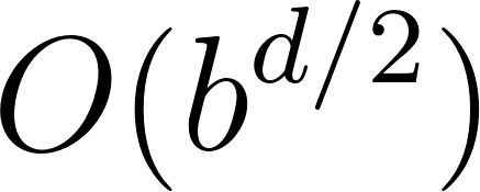 nodes. That square-root reduction effectively doubles the depth you can search in the same time, which is why strong game engines invest heavily in trying likely-best moves first. We return to exactly this idea, with real move-ordering heuristics, in the chess engine chapter.
We run all the search examples with one test program. Here we only show the output for the maze search example:
 1 $ scala-cli run .
 2 Starting compilation server
 3
 4 ==================================================
 5 Tic-Tac-Toe: Computer (X) vs Computer (O)
 6 ==================================================
 7
 8 X plays (0, 0):
 9 X . .
10 . . .
11 . . .
12
13 O plays (1, 1):
14 X . .
15 . O .
16 . . .
17
18 X plays (0, 1):
19 X X .
20 . O .
21 . . .
22
23 O plays (0, 2):
24 X X O
25 . O .
26 . . .
27
28 X plays (2, 0):
29 X X O
30 . O .
31 X . .
32
33 O plays (1, 0):
34 X X O
35 O O .
36 X . .
37
38 X plays (1, 2):
39 X X O
40 O O X
41 X . .
42
43 O plays (2, 1):
44 X X O
45 O O X
46 X O .
47
48 X plays (2, 2):
49 X X O
50 O O X
51 X O X
52
53 Draw!
The Tic-Tac-Toe result is the practical face of the minimax theorem. Two optimal players of a solved game can never beat each other, so a game between two copies of our engine always ends in a draw. The same search, given a game the opponent misplays, would convert every mistake into a win.
Running the Search Demos
We have already seen example output for the three examples. Now we look at the test harness code. The entry point in search/Main.scala coordinates all three search demos. First, it searches a small city graph:
 1   val graph = Graph(
 2     nodeDefs = List(
 3       ("Atlanta",    110, 520),
 4       ("Baltimore",  520, 360),
 5       ("Chicago",    310, 200),
 6       ("Denver",      75, 280),
 7       ("Erie",       480, 225),
 8       ("Fresno",      10, 400),
 9       ("Miami",        20, 800),
10       ("Seattle",     600, 100)
11     ),
12     edgeDefs = List(
13       ("Atlanta",   "Baltimore"),
14       ("Atlanta",   "Chicago"),
15       ("Atlanta",   "Denver"),
16       ("Atlanta",   "Miami"),
17       ("Baltimore", "Chicago"),
18       ("Chicago",   "Erie"),
19       ("Chicago",   "Seattle"),
20       ("Denver",    "Fresno"),
21       ("Denver",    "Chicago")
22     )
23   )
We already looked at the code to set up the maze and tic-tac-toe examples.
Running the project via scala-cli run . produces outputs we saw previously showing the DFS and BFS paths, the solved maze grid (drawing a path using .), and a complete optimal Tic-Tac-Toe game where two computers play each other to a draw.