A Chess Engine and AI Bot

Building a high-performance chess engine was a classic milestone in AI development. My lifelong interest in AI started when I played a Chess program on a PDP-8 and that motivated me to read Bertram Raphael’s book “The Thinking Computer: Mind Inside Matter” in 1977. I was hooked! Except for building a few very large scale distributed systems, most of my career has been AI-adjacent. I wrote the free Chess Chess program that Apple distributed with early Apple II computers.

In this chapter, we explore a Chess engine written in modern, idiomatic Scala 3.

The project compiles to efficient JVM bytecode, achieving searches of over 550,000+ NPS (Nodes Per Second) on standard developer laptops without any native dependencies.

All code is located in source-code/chess-game.

Chess has been the fruit fly of AI research since the field began. In 1950 Claude Shannon published “Programming a Computer for Playing Chess”, which laid out the architecture nearly every engine still uses: generate moves, evaluate positions with a scoring function, and search ahead through the tree of replies. Shannon drew the key distinction between a Type A strategy that searches every move to a fixed depth and a Type B strategy that searches selectively, spending effort only on promising lines. Around the same time Alan Turing wrote out a chess program by hand, executing it on paper because no machine could yet run it. The line runs through decades of work to IBM’s Deep Blue, which beat world champion Garry Kasparov in 1997.

The reason chess resists brute force is its sheer size. Shannon estimated the game-tree complexity at roughly 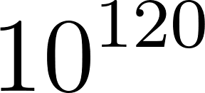(the “Shannon number”), and the number of legal positions is near 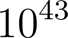. You cannot enumerate either. A search that generates 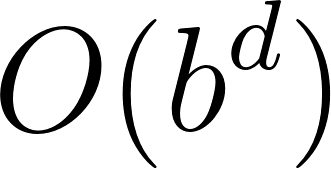nodes, with a branching factor 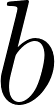near 35, becomes hopeless within a handful of plies. Every technique in this chapter exists to shrink that exponent: alpha-beta pruning cuts the base, transposition tables remove repeated work, move ordering makes the pruning bite, and the evaluation function lets us stop early with a sensible guess instead of searching to the end of the game.

A competitive chess engine is divided into three parts:

1. Board Representation & Move Generator: The rules of the game. It models the board and computes all legal moves for a given position.
2. Evaluation Function: The heuristics. It assigns a numerical score to a board position, indicating which side is winning.
3. Search Engine: The foresight. It explores the tree of possible future moves to select the best one.

To achieve maximum performance on the JVM, we avoid object allocation during the search. In chess-game/Engine.scala, the board is represented as an array of 64 bytes:

This design is a mailbox board: one array slot per square, each holding a small integer that encodes both the piece type and its color. The piece constants are chosen so the type lives in the low bits and the color in bits 8 and 16, so a single byte carries both and bit masks recover each part. Using a 64-element Array[Byte] makes square lookups O(1). We track active piece coordinates in mutable.Set[Int] collection lists for each player, allowing us to iterate over all active pieces in O(1) time rather than scanning all 64 squares.

The main alternative is a bitboard engine, which packs the 64 squares into a single 64-bit integer per piece type and uses bitwise operations to generate moves in parallel. Bitboards are faster still, and every top engine uses them, but they are harder to read and to get right. The mailbox array here keeps the code legible while the piece-set lists recover most of the speed you would otherwise lose scanning empty squares.

Calculating how slider pieces (Rooks, Bishops, Queens) and jump pieces (Knights, Kings) move is computationally expensive. We bypass this cost by precomputing move rays and targets at class initialization time inside the Precomputed object:

This is a classic time-for-space trade. The move geometry of a knight or a rook ray never changes, so we compute it once and read it back during search millions of times. Move generation also splits into two stages. First we build pseudo-legal moves, which follow each piece’s movement rules but may leave the king in check. Then we filter them down to legal moves by making each move, testing whether our own king is now attacked, and unmaking it. Splitting the work this way keeps the generator simple and pushes the expensive legality check onto only the moves we actually consider.

During search, makeMove modifies the board arrays in-place to avoid copying overhead, but it returns a lightweight BoardState snapshot containing the information needed to restore the state:

The matching unmakeMove rolls back mutations in O(1) time using the snapshot. This make/unmake pattern is what lets the engine walk a tree millions of nodes deep while allocating almost nothing. A naive engine that copied the whole board at every node would spend most of its time in the garbage collector. The snapshot holds only the small pieces of state that a move cannot recompute on its own: the en passant square, castling rights, the fifty-move counter, and the position hash. The board array itself is restored by reversing the specific squares the move touched.

To identify duplicate positions in the search tree (transpositions), we use Zobrist Hashing named after Albert Zobrist. A transposition is the same position reached by different move orders: play the same four moves in a different sequence and you often land on an identical board. If we recognize that, we can reuse the result we already computed instead of searching the position again. Zobrist published in 1970 a scheme that gives each position a 64-bit fingerprint. Each square-piece combination, active side, castling right, and en passant file is mapped to a unique random 64-bit number, and the position’s hash is the XOR of all the numbers that currently apply.

XOR is the perfect tool here for two reasons. It is its own inverse, so applying the same value twice cancels it, and it is associative and commutative, so the order of updates does not matter. When a move is made, we update the board’s hash incrementally: XOR out the piece on its old square and XOR it back in on its new square, keeping the hash accurate in O(1) time without rescanning the board:

The method above computes the hash from scratch, which we use once at startup and inside the Perft tests to confirm the incremental updates stayed correct. With 64 random bits the chance that two different positions collide is about 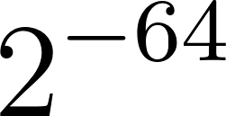, small enough to ignore in a search of a few million nodes.

The AI search in chess-game/AI.scala uses the Negamax formulation of minimax. Chess is a zero-sum game, so White’s gain is exactly Black’s loss. Negamax exploits this with the identity:

Rather than writing separate maximizing and minimizing branches, as the Tic-Tac-Toe minimax did in the search chapter, negamax always maximizes from the point of view of the side to move and negates the score returned by the recursive call. One line, val score = -search(board, depth - 1, -beta, -alpha), expresses the whole idea: your best reply, seen from the opponent, is their worst outcome, seen from you. The alpha-beta bounds are negated and swapped on the way down for the same reason.

Alpha-beta pruning itself works exactly as described in the search chapter: alpha is the best score the side to move can already guarantee, beta is the best the opponent can hold them to, and we cut off the moment alpha >= beta. The payoff is large. Perfect move ordering drops the node count from toward 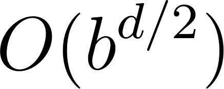, which nearly doubles the reachable depth. The rest of this section is about making that ordering as good as possible and reusing work across the tree:

The transposition table lookup at the top does two jobs. When the stored search went at least as deep as we need (ttEntry.depth >= depth), the cached score may be enough to return at once. When it is not deep enough, we still keep its bestMove to try first. The stored score carries a flag that marks it as one of three kinds: an exact value, a lower bound, or an upper bound. A cutoff produces a bound rather than an exact value, because pruning stops the search before it has proven the true score, only that the score is at least or at most some number. The lookup honors that: an exact value returns directly, a lower bound returns only if it already beats beta, and an upper bound returns only if it already fails below alpha. Mate scores need one extra correction. A checkmate is scored relative to the root, so before we store or reuse it we shift it by maxDepth - depth to express the mate as a distance from the current node instead.

• Transposition Table: We cache previously searched positions in a JVM primitive-optimized mutable.LongMap to prevent object boxing and skip re-searching known branches. A plain Map[Long, TTEntry] would box every 64-bit key into a heap object; LongMap stores the primitive Long directly, which matters when the table holds hundreds of thousands of entries. The engine caps the table at 500,000 entries and clears it when it grows past that, trading a little cached knowledge for bounded memory.
• Iterative Deepening: We search progressively from depth 1 up to the target depth. This sounds wasteful, but it is nearly free. Because the tree grows by a factor of per ply, the final depth dominates the total cost: the sum is only about 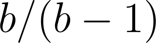times 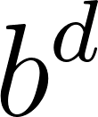, so re-searching the shallow layers adds a small constant overhead. In return we gain two things: the best move from each shallow search orders the next, deeper search so that alpha-beta cuts far more branches, and the engine can stop at any time with the best move found so far.
• Quiescence Search: A fixed-depth search suffers the horizon effect, first named by Hans Berliner: a bad move can look good because a refuting capture happens one ply past the search limit. To fix this, at depth 0 we do not evaluate immediately. Instead we extend the search over captures and promotions until the position is “quiet”, so we never evaluate a board in the middle of a trade. The quiescence search also uses a stand-pat score, the static evaluation of the current position, as a lower bound, on the assumption that the side to move is not forced to capture.
• Smart Move Ordering: We order moves by looking at Transposition Table moves first, then captures using MVV-LVA (Most Valuable Victim, Least Valuable Attacker), promotion scores, and positional values from Piece-Square Tables (PSTs). MVV-LVA captures the intuition that grabbing a queen with a pawn is more likely to be strong than grabbing a pawn with a queen, so it tries the former first. The moveValue function encodes this ordering as a single integer priority.

When the search reaches its depth limit it needs a number, a static estimate of who stands better without looking further. Our evaluation combines two ideas that go back to Shannon’s original paper. The first is material: each piece has a value in centipawns (a pawn is 100, a knight 320, a bishop 330, a rook 500, a queen 900). The king is set to 20000, not because it can be traded but so its safety dominates every other term. The second is position: a knight on a central square controls more board than one in a corner, so we add a bonus that depends on where each piece sits. Those bonuses live in Piece-Square Tables (PSTs).

The bot evaluates coordinate maps differently depending on the stage of the game. For example, during the middlegame, it rewards keeping the King safe in the corners; during the endgame, it uses a centralization table to pull the King into active play:

Two implementation details make the tables compact. The tables are written from White’s point of view, so to score a Black piece the code reads the table at the mirrored square sq ^ 56. XOR with 56 flips the three rank bits of a square index, reflecting the board top to bottom, which is exactly the symmetry between White’s and Black’s home ranks. That single trick lets one table serve both colors. The engine also picks the king table by asking isEndgame, which sums the non-pawn material and switches to the centralization table once it drops below a threshold. The final score is returned from the point of view of the side to move (if (board.turn == WHITE) score else -score), which is precisely the convention negamax expects.

You can play against the bot or watch it play against itself using CLI.scala. Launch it with:

The CLI features an interactive ANSI board rendering and a sidebar tracking the game statistics:

To validate the move generator and check the integrity of Zobrist hashing, run the Perft verification suite. Perft (performance test) counts the exact number of leaf nodes reachable at a given depth. Those counts are known constants for the starting position, so any bug in move generation, in make/unmake, or in the incremental hash shows up immediately as a wrong total. The test also recomputes the Zobrist hash from scratch after every move and compares it against the incrementally updated value, catching hash bugs the node count alone would miss:

This counts every reachable terminal state at deep levels, ensuring correctness against official chess standards:

The 20, 400, and 8902 figures are the standard reference values every chess programmer checks against. Matching them exactly gives strong evidence that the rules engine, from castling and en passant to promotion and check detection, is correct. The nodes-per-second figure alongside them is the raw search speed, the same metric used to compare production engines, and the number that all the optimizations in this chapter work to raise.