Backpropagation Neural Networks from Scratch
While modern Machine Learning often relies on massive libraries like PyTorch or TensorFlow, implementing a neural network from scratch is a powerful way to truly master the underlying mathematics of deep learning. Deep learning networks have many layers but the smaller two or three layer models as we implement here are still useful: in the 1980s at SAIC, I wrote a simple backpropagation neural model that we used in a bomb detector for the FAA, same technology!
In this chapter, we build a backpropagation neural network with one hidden layer in pure Scala 3, with zero dependencies.
Unlike traditional object-oriented implementations (which mutate weight arrays in place), we use a functional style: the network state is encapsulated in an immutable case class, and training methods return an updated copy of the network.
All code is in source-code/neural-networks.
A Short History: Why We Need Hidden Layers
The artificial neuron dates to 1943, when Warren McCulloch and Walter Pitts modeled a nerve cell as a unit that sums its inputs and fires if the sum passes a threshold. In 1958 Frank Rosenblatt turned this into the perceptron, a trainable single-layer classifier. Progress stalled in 1969 when Marvin Minsky and Seymour Papert proved a hard limit in their book Perceptrons: a single layer can only separate classes with a straight line (a hyperplane), so it cannot learn the XOR function, whose true cases sit on opposite corners of a square. This result cooled research for years.
The way out is a hidden layer. Stack a second layer of neurons between input and output and the network can carve the input space into regions that no single line could, so XOR becomes learnable. The missing piece was a training method for the hidden weights. It arrived in 1986, when David Rumelhart, Geoffrey Hinton, and Ronald Williams popularized backpropagation, an efficient way to compute how every weight in a multi-layer network affects the error. That algorithm is what we build here, and it remains the engine under every modern deep network.
Hidden layers only help if the neurons are nonlinear. A neuron computes a weighted sum, and the sum of sums is still just a sum: stack any number of purely linear layers and the whole network collapses to a single linear map, no more powerful than one perceptron. Inserting a nonlinear activation function after each layer breaks this collapse and lets depth add real expressive power. In fact the universal approximation theorem (George Cybenko in 1989, Kurt Hornik in 1991) shows that a single hidden layer with enough nonlinear units can approximate any continuous function to any accuracy. Our XOR network is the smallest interesting instance of that theorem.
Neural Network Representation
Our network is defined in neural-networks/NeuralNetwork.scala as a case class wrapping the dimensional configurations and weight matrices:
1 case class NeuralNetwork(
2     numInputs: Int,
3     numHidden: Int,
4     numOutputs: Int,
5     w1: Array[Array[Float]],
6     w2: Array[Array[Float]],
7     learningRate: Float = 0.5f
8 ):
Here, w1 represents the weights from the input layer to the hidden layer, and w2 represents the weights from the hidden layer to the output layer. Each is a matrix: w1 has shape  and
w2 has shape  . The whole network is nothing more than these two matrices plus their sizes, which is why the case class captures the entire model state.
To keep the code minimal, this network omits bias terms, the per-neuron constants that let an activation shift left or right independent of its inputs. Production networks always include them, and we would add a bias by giving each layer one extra input fixed at 1.0. The XOR problem is still learnable without explicit biases because the four hidden units can cooperate to shape the decision boundary, as the demo output later confirms.
Activation Function
We use the standard Sigmoid function to introduce non-linearity into the network, allowing it to learn non-linear decision boundaries:
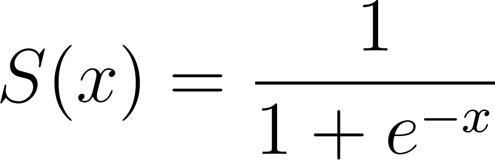
The sigmoid squashes any real number into the range 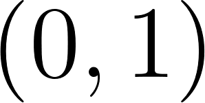 , which makes its output easy to read as a probability or a soft on/off signal. Its derivative has a particularly convenient closed form when expressed in terms of the activated value
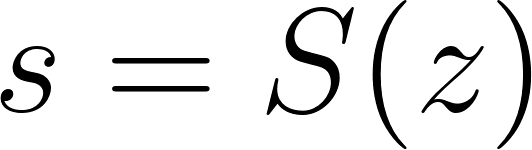 :

This identity is the reason sigmoid was the default for decades: during backpropagation we already have the activation  in hand, so computing the gradient costs one multiply and one subtract, with no second call to
exp. In code, we define the sigmoid and its derivative:
1 object NeuralNetwork:
2   def sigmoid(x: Float): Float =
3     (1.0f / (1.0f + math.exp(-x).toFloat))
4
5   /** Derivative of sigmoid where the input is already activated (s = sigmoid(z)). */
6   def sigmoidPrime(s: Float): Float =
7     s * (1.0f - s)
The convenient derivative comes at a cost worth knowing. Notice that 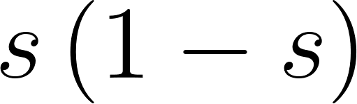 peaks at only
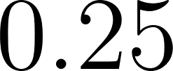 and falls to nearly zero when is close to 0 or 1. In a deep network these small factors multiply together and the gradient shrinks toward nothing as it flows back through many layers, the vanishing gradient problem. This is why modern deep networks favor the ReLU activation,
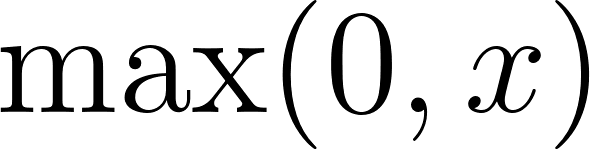 , whose gradient is a flat 1 for positive inputs. For a shallow network like ours, sigmoid works fine.
Feedforward Pass
The forward pass runs input values through the network to compute the hidden activations and final outputs. We multiply the input vector by the weight matrix, sum them, and apply the sigmoid function:
 1   /** Forward pass: returns (hiddenActivations, outputActivations). */
 2   def forward(inputs: Array[Float]): (Array[Float], Array[Float]) =
 3     // input → hidden
 4     val hidden = Array.ofDim[Float](numHidden)
 5     for i <- 0 until numInputs; h <- 0 until numHidden do
 6       hidden(h) += inputs(i) * w1(i)(h)
 7     for h <- 0 until numHidden do
 8       hidden(h) = NeuralNetwork.sigmoid(hidden(h))
 9
10     // hidden → output
11     val outputs = Array.ofDim[Float](numOutputs)
12     for h <- 0 until numHidden; o <- 0 until numOutputs do
13       outputs(o) += hidden(h) * w2(h)(o)
14     for o <- 0 until numOutputs do
15       outputs(o) = NeuralNetwork.sigmoid(outputs(o))
16
17     (hidden, outputs)
18
19   /** Run a single input through the network and return the outputs. */
20   def recall(inputs: Array[Float]): Array[Float] = forward(inputs)._2
Each layer performs the same two steps: a matrix-vector product followed by an element-wise nonlinearity. The nested loop hidden(h) += inputs(i) * w1(i)(h) is a hand-written matrix multiply; a library like PyTorch would express the whole thing as sigmoid(W1 · x) and dispatch it to optimized BLAS routines, but the arithmetic is identical. We return both the hidden and output activations, because backpropagation needs the hidden activations again to compute the gradient, and recomputing them would waste work.
Backpropagation and Weight Updates
Training means finding weights that make the outputs match the targets. We frame this as minimizing an error function, the squared difference between target and output summed over the output neurons:
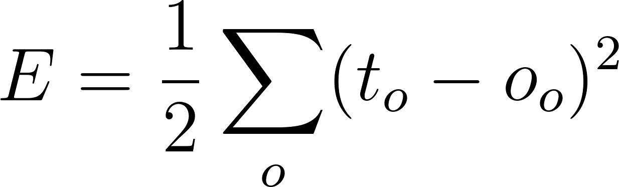
The error  is a surface over the space of all weights, and we want its lowest point. Gradient descent finds it by repeatedly stepping each weight a little in the direction that most reduces , which is the negative gradient
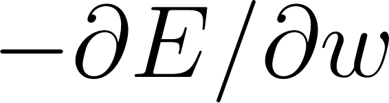 . The only hard part is computing that gradient for a weight buried in the hidden layer, and this is exactly what backpropagation does using the chain rule of calculus: the error’s sensitivity to a hidden weight is the product of sensitivities along the path from that weight to the output. Working the chain rule through our two layers gives the three familiar update rules:
- Output Error: Calculate the difference between targets and outputs, multiplied by the derivative of the activation function:

- Hidden Error: Propagate the error backward through the weights
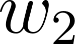 to the hidden layer. Each hidden neuron gets a share of the blame proportional to how strongly it fed each output:
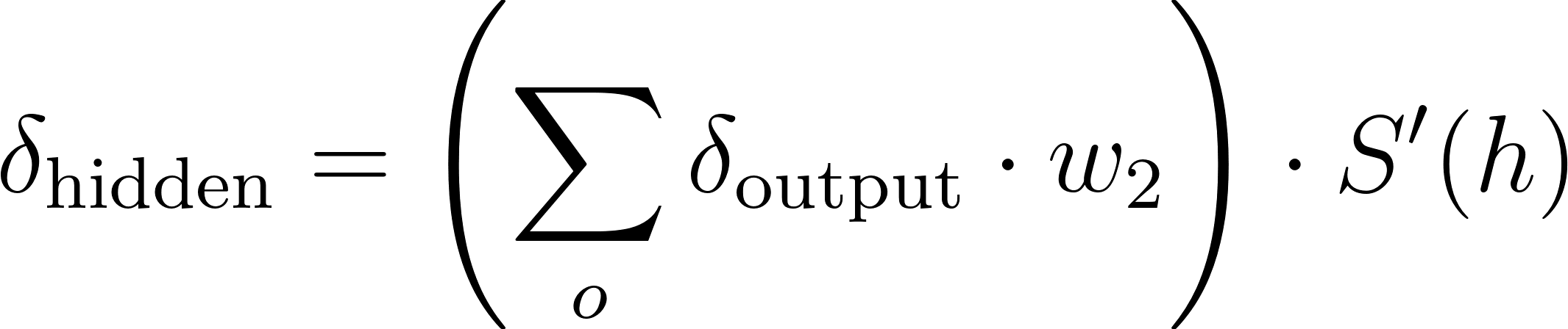
- Weight Update: Create new weight matrices by adding the product of the errors, the activations, and the learning rate
 :

The 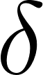 terms are the heart of the algorithm. Each one measures how much a neuron’s total input should change to lower the error, and the weight update simply moves each weight in proportion to the error at its downstream neuron and the activation at its upstream neuron. The learning rate scales every step: too small and training crawls, too large and the updates overshoot the minimum and the error can oscillate or diverge. Our demo uses
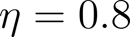 , which is aggressive but works for this tiny problem.
Here is how we implement this functionally in Scala:
 1   /** Train on one example. Returns (updatedNetwork, error). */
 2   def trainOne(inputs: Array[Float], targets: Array[Float]): (NeuralNetwork, Float) =
 3     val (hidden, outputs) = forward(inputs)
 4
 5     // output errors
 6     val outputErrors = Array.ofDim[Float](numOutputs)
 7     for o <- 0 until numOutputs do
 8       outputErrors(o) = (targets(o) - outputs(o)) * NeuralNetwork.sigmoidPrime(outputs(o))
 9
10     // hidden errors (backprop)
11     val hiddenErrors = Array.ofDim[Float](numHidden)
12     for h <- 0 until numHidden do
13       var sum = 0f
14       for o <- 0 until numOutputs do sum += outputErrors(o) * w2(h)(o)
15       hiddenErrors(h) = sum * NeuralNetwork.sigmoidPrime(hidden(h))
16
17     // update weights (create new arrays)
18     val newW2 = Array.tabulate(numHidden, numOutputs): (h, o) =>
19       w2(h)(o) + learningRate * outputErrors(o) * hidden(h)
20     val newW1 = Array.tabulate(numInputs, numHidden): (i, h) =>
21       w1(i)(h) + learningRate * hiddenErrors(h) * inputs(i)
22
23     val error = (0 until numOutputs).map(o => math.abs(targets(o) - outputs(o))).sum
24     (copy(w1 = newW1, w2 = newW2), error)
The code maps one-to-one onto the three equations. Notice that sigmoidPrime receives the already-activated value (outputs(o), hidden(h)), which is why the derivative is written as s * (1 - s) rather than in terms of the raw pre-activation. The functional design shows up in the last line: instead of mutating w1 and w2 in place, we build new arrays with Array.tabulate and return a fresh NeuralNetwork via copy. This makes the network immutable and each training step a pure function from old network to new network, which is easy to reason about and test. The trade-off is allocation: we create two new weight matrices per example. For large networks you would mutate in place to avoid that cost, but for teaching the algorithm the clarity is worth it. Note also that the returned error uses the absolute difference |t - o| purely as a human-readable progress metric; the value the training actually minimizes is the squared error whose gradient produced the delta rules above.
Because trainOne updates the weights after every single example, this is stochastic (online) gradient descent. The alternative, batch gradient descent, would accumulate the gradients over all examples and apply one averaged update per pass. Online updates are noisier but often converge faster and can escape shallow dips in the error surface. We also write a helper to train the network over a list of training examples for an entire epoch, folding the updated network through the inputs:
1   /** Train on a list of (input, target) pairs for one epoch. */
2   def trainEpoch(examples: List[(Array[Float], Array[Float])]): (NeuralNetwork, Float) =
3     var net = this
4     var totalError = 0f
5     for (inputs, targets) <- examples do
6       val (updated, err) = net.trainOne(inputs, targets)
7       net = updated
8       totalError += err
9     (net, totalError / examples.size)
One subtlety of training deserves mention: the random starting weights. We initialize weights to small random values in 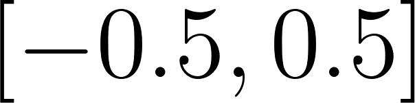 rather than to zero. If every weight started equal, every hidden neuron would compute the same output and receive the same gradient, so they would stay identical forever and the hidden layer would collapse to a single neuron. Random initialization breaks this symmetry and lets each hidden unit specialize.
Demo: Learning the XOR Gate
The XOR logical gate is a classic AI benchmark because it is not linearly separable. As Minsky and Papert showed, a single-layer perceptron cannot learn it, which makes the hidden layer necessary and makes XOR the perfect smallest test of a real multi-layer network.
Our demo program initializes a network with 2 inputs, 4 hidden units, and 1 output, then trains it on the XOR truth table over 5000 epochs:
 1 @main def neuralNetworkDemo(): Unit =
 2   val xorExamples = List(
 3     (Array(0f, 0f), Array(0f)),
 4     (Array(0f, 1f), Array(1f)),
 5     (Array(1f, 0f), Array(1f)),
 6     (Array(1f, 1f), Array(0f))
 7   )
 8
 9   var net = NeuralNetwork.random(
10     numInputs = 2, numHidden = 4, numOutputs = 1,
11     learningRate = 0.8f
12   )
13
14   val numEpochs = 5000
15   for epoch <- 1 to numEpochs do
16     val (updated, error) = net.trainEpoch(xorExamples)
17     net = updated
18     if epoch % 500 == 0 || epoch == 1 then
19       println(f"  Epoch $epoch%5d  avg error: $error%.6f")
20
21   println("\nTrained network results:")
22   for (input, target) <- xorExamples do
23     val output = net.recall(input)
24     println(f"  Input: [${input(0)}%.0f, ${input(1)}%.0f]  " +
25             f"Target: ${target(0)}%.0f  Output: ${output(0)}%.4f")
Running this code with scala-cli run . outputs:
 1 ==================================================
 2 Neural Network: Learning XOR
 3 ==================================================
 4   Epoch     1  avg error: 0.505372
 5   Epoch   500  avg error: 0.380295
 6   Epoch  1000  avg error: 0.101740
 7   Epoch  1500  avg error: 0.046399
 8   Epoch  2000  avg error: 0.030560
 9   Epoch  2500  avg error: 0.023247
10   Epoch  3000  avg error: 0.018939
11   Epoch  3500  avg error: 0.016075
12   Epoch  4000  avg error: 0.014022
13   Epoch  4500  avg error: 0.012476
14   Epoch  5000  avg error: 0.011265
The error curve tells the story of gradient descent. The first 500 epochs barely move: the network sits on a nearly flat part of the error surface while the hidden units slowly differentiate. Around epoch 1000 the error drops sharply as the network discovers a useful internal representation, then the improvement tapers as it settles into the minimum. This slow start followed by a fast drop is typical of small networks learning a nonlinear function. The final results confirm the network learned XOR:
1 Trained network results:
2   Input: [0, 0]  Target: 0  Output: 0.0104
3   Input: [0, 1]  Target: 1  Output: 0.9892
4   Input: [1, 0]  Target: 1  Output: 0.9890
5   Input: [1, 1]  Target: 0  Output: 0.0124
As the output shows, the final errors drop to nearly 1%, and the model correctly outputs values extremely close to the targets. The network never sees the rule for XOR; it discovers, purely from four examples and the gradient of its own error, a set of weights that computes a function no single-layer perceptron ever could.