A Tiny Transformer from Scratch
The neural networks chapter built a one-layer perceptron by hand. This chapter climbs one rung higher and builds the architecture that powers modern language models: a transformer. Ours is character-level, has one attention block with two heads, and trains on a CPU in a few seconds. It contains every essential piece of a GPT: token embeddings, causal self-attention, multi-head projection, RMSNorm, a feed-forward network, an output head, cross-entropy loss, and a scalar autograd engine you can read in full.
The goal is not scale. It is transparency. Every parameter is a single Double carrying its own gradient, so there is no hidden machinery between the equations and the code. Once you have watched a thousand-parameter transformer learn to spell hello, the gap to a billion-parameter model is one of size and data, not of kind.
All code is in source-code/micro-transformer. Credit goes to Andrej Karpathy’s microGPT, a minimal dependency-free GPT written in Python, whose design this port follows.
Why Attention Replaced Recurrence
A language model is a next-token predictor. Given a sequence of tokens, it produces a probability for every token in the vocabulary, and training pushes up the probability of the token that actually came next.
Before transformers, the standard tool for this job was the recurrent neural network (RNN), and later the LSTM. An RNN reads a sequence one step at a time and carries a hidden state forward: at each step the hidden state is a function of the previous hidden state and the current input. This design has three costs. First, it is inherently sequential, so a GPU cannot process all positions at once. Second, information from the start of a long sequence must survive being overwritten at every intermediate step, so long-range dependencies are hard to learn. Third, gradients flow back through the same chain of steps, and repeated multiplication shrinks them, the vanishing gradient problem again.
Attention removes all three costs at once. Instead of a single running state, every position keeps its own vector and is allowed to look directly at every earlier position. At each position, the model asks a question (a query), compares it against a label attached to every earlier position (a key), and uses the match scores to take a weighted average of the earlier positions’ content (the values). The path between any two positions is one step, not many, and all positions can be computed in parallel. This mechanism, introduced in the 2017 paper “Attention Is All You Need” by Vaswani and colleagues, is the core of the transformer.
For a language model we must be careful that a position cannot see the future, or training would be trivial: the model would just copy the answer. We therefore mask the scores so that position  may attend only to positions
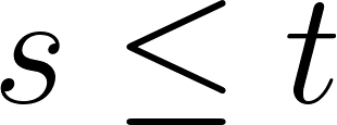 . This is called causal attention, and it is what makes the model usable for generation.
A full transformer stacks many blocks, each combining attention with a small feed-forward network. Our version uses a single block with two attention heads, small enough that the whole forward pass is a few dozen lines.
A Tiny Corpus and Character Tokens
The training text sits in source-code/micro-transformer/data/corpus.txt, sixteen short lines of repeating toy English:
 1 hello world
 2 hello scala
 3 hello there
 4 hello again world
 5 scala runs on the jvm
 6 the jvm runs scala code
 7 hello jvm world
 8 small models learn small texts
 9 hello small model
10 the model reads hello world
11 attention links the words
12 words link to words
13 hello attention model
14 the tiny net trains fast
15 fast training on small texts
16 hello tiny transformer
We tokenize at the character level. That avoids a separate tokenizer and keeps the vocabulary tiny, at the cost of longer sequences. The demo lowercases the text, collects the distinct characters, sorts them, and builds two lookup maps, stoi (string to integer) and itos (integer to string):
1 val text = Files.readString(Paths.get("data/corpus.txt")).toLowerCase
2 val chars = text.distinct.sorted
3 val stoi = chars.zipWithIndex.toMap
4 val itos = stoi.map(_.swap)
5 val ids = text.map(stoi).toArray
Because the raw file is read whole, the newline character is part of the text and becomes a token. The vocabulary has 24 symbols: the newline, the space, and 22 letters.
Training examples come from a sliding window. With a block size of 8, every offset in the text yields an input of 8 characters and a target of the same 8 characters shifted one position to the left, so each input character is trained to predict the one that follows it:
1 input : hello wo
2 target: ello wor
The transformer sees all 8 positions at once, and every position contributes a prediction. This is much more efficient than the recurrent approach, which would update the weights once per character.
The Autograd Engine
Training requires gradients: for every parameter, how much does the loss change when that parameter changes? We compute them by reverse-mode automatic differentiation, also called backpropagation. The idea is to record every operation as a node in a graph during the forward pass, then walk the graph backward applying the chain rule.
Each node is a Value, holding a number, a gradient, its parent nodes, and a closure that knows how to push gradient to those parents. The full engine is in Autograd.scala:
 1 //> using scala 3.6.4
 2 // Copyright 2026 Mark Watson. All rights reserved.
 3
 4 package microtransformer
 5
 6 import scala.collection.mutable
 7
 8 // Scalar autograd engine. Port of the Value struct and v+/v*/vpow/
 9 // vlog/vexp/vrelu/backward code in microgpt.lisp.
10 class Value(var data: Double, var grad: Double = 0.0):
11   private var children: Set[Value] = Set.empty
12   private var backwardFn: () => Unit = () => ()
13
14   private def result(d: Double, kids: Set[Value], back: Value => () => Unit): Value =
15     val v = new Value(d)
16     v.children = kids
17     v.backwardFn = back(v)
18     v
19
20   def +(other: Value): Value =
21     val a = this; val b = other
22     result(data + b.data, Set(a, b), out => () => { a.grad += out.grad; b.grad += out.grad })
23   def *(other: Value): Value =
24     val a = this; val b = other
25     result(data * b.data, Set(a, b), out => () => { a.grad += b.data * out.grad; b.grad += a.data * out.grad })
26   def pow(p: Double): Value =
27     val a = this
28     result(math.pow(data, p), Set(a), out => () => a.grad += p * math.pow(a.data, p - 1) * out.grad)
29   def exp(): Value =
30     val a = this
31     val e = math.exp(data)
32     result(e, Set(a), out => () => a.grad += e * out.grad)
33   def log(): Value =
34     val a = this
35     result(math.log(data), Set(a), out => () => a.grad += out.grad / a.data)
36   def relu(): Value =
37     val a = this
38     result(math.max(0.0, data), Set(a), out => () => a.grad += (if a.data > 0.0 then out.grad else 0.0))
39   def unary_- : Value = this * Value(-1.0)
40   def -(other: Value): Value = this + (-other)
41   def /(other: Value): Value = this * other.pow(-1.0)
42
43   def backward(): Unit =
44     val topo = mutable.ListBuffer[Value]()
45     val seen = mutable.Set[Value]()
46     def build(v: Value): Unit =
47       if !seen.contains(v) then
48         seen.add(v)
49         v.children.foreach(build)
50         topo.append(v)
51     build(this)
52     grad = 1.0
53     topo.reverse.foreach(_.backwardFn())
54
55 object Value:
56   def apply(d: Double): Value = new Value(d)
57
58   // Softmax over one row of Values. Each output holds the graph.
59   def softmax(logits: Seq[Value]): Seq[Value] =
60     val m = logits.map(_.data).max
61     val exps = logits.map(v => (v - Value(m)).exp())
62     val s = exps.reduce(_ + _)
63     exps.map(_ / s)
Each operator follows the same recipe: compute the output number, remember which nodes produced it, and store a backward closure. The derivative rules are the ones from a first calculus course:
- Addition passes the incoming gradient through unchanged:
 and
 .
- Multiplication uses the product rule:
 and
 .
- A power uses the power rule,
 .
- The exponential is its own derivative,
 .
- The logarithm has derivative
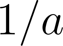 .
- ReLU passes the gradient only where its input was positive.
Subtraction and division need no rules of their own. They are expressed in terms of the primitives: a - b becomes a + (-b), and a / b becomes a * b^{-1}. This keeps the engine small and shows how a complete op set can be built from a handful of pieces.
The result helper is where the graph is wired. Note the type of the backward function: Value => () => Unit. It is a function that takes the output node and returns a thunk that will later read that output’s gradient. Writing it this way matters. The closure must read out.grad, the gradient arriving at the node it produced, not the gradient of an operand. The chain rule multiplies the local derivative by that incoming gradient, so capturing the wrong value produces wrong gradients, and the test below catches the error immediately.
The backward method performs a topological sort with a depth-first walk: it visits all children of a node before recording the node itself, so the list runs from inputs to output. Reversing that list processes the output first and each parameter last, which guarantees that a node’s gradient is fully accumulated from all of its consumers before its own backward step runs. The loss node is seeded with a gradient of 1.0, the convention that 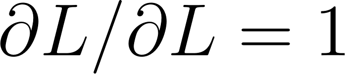 .
softmax is written in terms of the same primitives, so its outputs stay connected to the graph and no extra backward rule is needed. Subtracting the row maximum before exponentiating is a numerical safeguard: 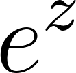 overflows for even moderately large
 , and shifting every logit by the same constant leaves the softmax unchanged while keeping the exponents near zero.
The Transformer Block
The model lives in MicroGPT.scala. It holds thirteen parameter groups, all as Value scalars: the token embedding table, per-head query, key, and value maps, an attention output projection, two RMSNorm gains, two MLP weight matrices with their biases, and the output head with its bias.
1 class MicroGPT(
2     val vocabSize: Int,
3     val blockSize: Int,
4     nEmbd: Int = 8,
5     nHead: Int = 2,
6     hidden: Int = 16,
7     seed: Long = 7
8 ):
The defaults are deliberately tiny. The embedding width is  , split across
 heads, so each head has dimension
 . The MLP expands to
 and contracts back to
 . With a vocabulary of 24 and a block size of 8, the whole network has exactly 960 parameters.
Initialization draws weights from a Gaussian with a small standard deviation, and the two RMSNorm gains start near  . Small random weights break symmetry, the same reason the neural network chapter used them: identical units would receive identical gradients and stay identical forever.
 1 private val rng = new scala.util.Random(seed)
 2 private def rand(rows: Int, cols: Int, scale: Double = 0.5): Array[Array[Value]] =
 3   Array.fill(rows, cols)(Value(rng.nextGaussian() * scale))
 4 private def randVec(n: Int): Array[Value] =
 5   Array.fill(n)(Value(1.0 + rng.nextGaussian() * 0.05))
 6
 7 val tokenEmbed: Array[Array[Value]] = rand(vocabSize, nEmbd)
 8 val wq: Array[Array[Array[Value]]] = Array.fill(nHead)(rand(nEmbd / nHead, nEmbd, 0.3))
 9 val wk: Array[Array[Array[Value]]] = Array.fill(nHead)(rand(nEmbd / nHead, nEmbd, 0.3))
10 val wv: Array[Array[Array[Value]]] = Array.fill(nHead)(rand(nEmbd / nHead, nEmbd, 0.3))
11 val wo: Array[Array[Value]] = rand(nEmbd, nEmbd, 0.3)
12 val ln1: Array[Value] = randVec(nEmbd)
13 val w1: Array[Array[Value]] = rand(nEmbd, hidden, 0.3)
14 val b1: Array[Value] = Array.fill(hidden)(Value(0.0))
15 val w2: Array[Array[Value]] = rand(hidden, nEmbd, 0.3)
16 val b2: Array[Value] = Array.fill(nEmbd)(Value(0.0))
17 val ln2: Array[Value] = randVec(nEmbd)
18 val wOut: Array[Array[Value]] = rand(vocabSize, nEmbd, 0.3)
19 val bOut: Array[Value] = Array.fill(vocabSize)(Value(0.0))
The parameters method flattens all of them into one sequence, which the optimizer and the gradient test both iterate:
1 def parameters: Seq[Value] =
2   tokenEmbed.flatten.toSeq ++ wq.flatten.flatten ++ wk.flatten.flatten ++
3     wv.flatten.flatten ++ wo.flatten ++ ln1 ++ w1.flatten ++ b1 ++
4     w2.flatten ++ b2 ++ ln2 ++ wOut.flatten ++ bOut
Two small helpers carry most of the arithmetic. matVec multiplies a matrix by a vector, and rmsNorm normalizes a vector:
1 private def matVec(m: Array[Array[Value]], x: Array[Value]): Array[Value] =
2   m.map(row => row.zip(x).map { case (a, b) => a * b }.reduce(_ + _))
3
4 private def rmsNorm(x: Array[Value], g: Array[Value]): Array[Value] =
5   val ms = x.map(v => v * v).reduce(_ + _) / Value(x.size.toDouble)
6   val inv = (ms + Value(1e-6)).pow(-0.5)
7   x.zip(g).map { case (v, s) => v * inv * s }
RMSNorm stands for root-mean-square normalization. It divides each element by the root mean square of the vector and then scales it by a learned gain  :

The 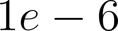 epsilon keeps the denominator away from zero. Unlike LayerNorm, RMSNorm does not subtract the mean, which makes it cheaper and works about as well in practice. The gain vector is learned, so the network can undo the normalization where that helps.
The forward method is the whole architecture in one function:
 1 // Forward pass over one block. Returns per-position logits.
 2 def forward(ids: Array[Int]): Array[Array[Value]] =
 3   var x = ids.map(tokenEmbed(_))
 4   // Causal single-layer attention with residual.
 5   val headDim = nEmbd / nHead
 6   val attended = x.indices.map { t =>
 7     val outs = (0 until nHead).map { h =>
 8       val q = matVec(wq(h), x(t))
 9       val ks = (0 to t).map(s => matVec(wk(h), x(s)))
10       val vs = (0 to t).map(s => matVec(wv(h), x(s)))
11       val scores = ks.map(k => q.zip(k).map { case (a, b) => a * b }.reduce(_ + _) / Value(math.sqrt(headDim)))
12       val weights = Value.softmax(scores)
13       (0 until headDim).map { i =>
14         weights.zip(vs).map { case (w, v) => w * v(i) }.reduce(_ + _)
15       }.toArray
16     }
17     outs.foldLeft(Array.empty[Value])(_ ++ _)
18   }.toArray
19   x = x.zip(attended).map { case (xi, ai) =>
20     val proj = matVec(wo, ai)
21     xi.zip(proj).map { case (a, b) => a + b }
22   }
23   x = x.map(rmsNorm(_, ln1))
24   // MLP with residual.
25   x = x.zip(x.map { xi =>
26     val h = matVec(w1, xi).zip(b1).map { case (a, b) => (a + b).relu() }
27     matVec(w2, h).zip(b2).map { case (a, b) => a + b }
28   }).map { case (a, b) => a.zip(b).map { case (p, q) => p + q } }
29   x = x.map(rmsNorm(_, ln2))
30   x.map(xi => matVec(wOut, xi).zip(bOut).map { case (a, b) => a + b })
We will take it stage by stage.
Embeddings
The first line turns token ids into vectors by looking up a row of the embedding table. tokenEmbed has shape  , so each character becomes a point in 8-dimensional space that the network learns to place.
The line deserves a note, because an earlier version of it hid a bug. It used to read:
1 var x = ids.map(tokenEmbed(_).map(v => Value(v.data) + Value(0.0)))
That copy creates a fresh leaf node holding the same number, so the new node has no link back to the embedding table. Gradient stops at the copy, and the embedding table, though listed among the parameters, never receives a nonzero gradient and never changes. A quick check confirms it: after a backward pass the sum of absolute embedding gradients is exactly  . Using the table rows directly, as above, lets the gradient flow and turns the embeddings into learned parameters. Because the same character can appear at several positions in a block, its row accumulates gradient from each position, which is exactly what we want.
Causal Self-Attention
Attention is the heart of the model. For each position and each head 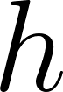 , the code computes three projections of the input vector
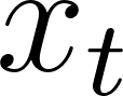 :
1 val q = matVec(wq(h), x(t))
2 val ks = (0 to t).map(s => matVec(wk(h), x(s)))
3 val vs = (0 to t).map(s => matVec(wv(h), x(s)))
The query  asks what this position is looking for. The keys
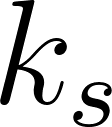 describe what each earlier position offers. The values
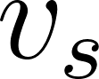 are the content that will be mixed together. Each projection is its own learned matrix, of shape
 , so all three can learn different features of the same input.
The match score between the query at and the key at  is their dot product, scaled by the square root of the head dimension:
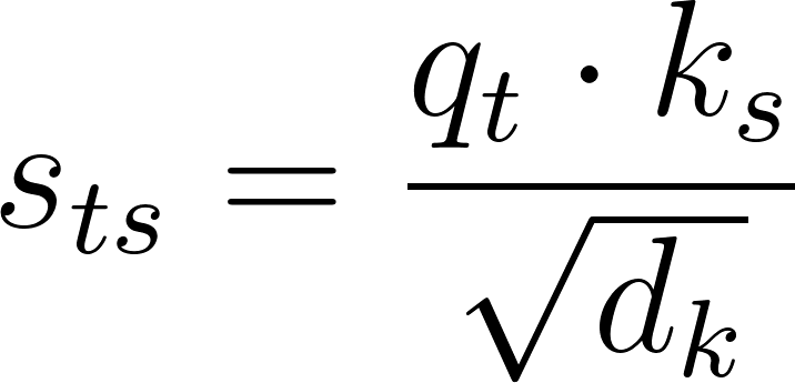
The scaling matters. A dot product of two 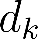 -dimensional vectors grows with when the components are roughly independent, and large logits push softmax into a regime where one weight is nearly
 and the rest nearly
 . The gradients there are tiny, so learning stalls. Dividing by
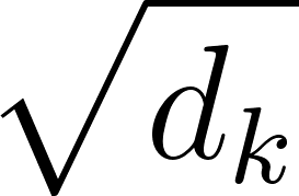 keeps the scores at a workable scale.
The scores are passed through softmax to become attention weights that sum to one, and then the output is the weighted average of the values:
1 val scores = ks.map(k => q.zip(k).map { case (a, b) => a * b }.reduce(_ + _) / Value(math.sqrt(headDim)))
2 val weights = Value.softmax(scores)
3 (0 until headDim).map { i =>
4   weights.zip(vs).map { case (w, v) => w * v(i) }.reduce(_ + _)
5 }.toArray
In full, one attention head computes:
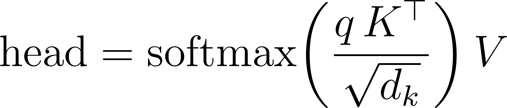
Causality is enforced by construction, not by a mask matrix. The inner loop builds keys and values with (0 to t), so position simply never sees positions after itself. That is why the model can be used to generate text one character at a time: at each step it only ever looks left.
Multiple Heads
A single attention head can only average the past one way. Multi-head attention runs several heads in parallel, each with its own query, key, and value matrices, so different heads can attend to different kinds of relationships. With and , each head works in a 4-dimensional subspace.
The heads are computed independently and then concatenated back to width 8:
1 outs.foldLeft(Array.empty[Value])(_ ++ _)
The concatenated result is projected back to the model width by wo and added to the original input:
1 x = x.zip(attended).map { case (xi, ai) =>
2   val proj = matVec(wo, ai)
3   xi.zip(proj).map { case (a, b) => a + b }
4 }
That addition is a residual connection. It gives the gradient a direct path around the attention computation, which makes deep networks trainable and lets each block learn a refinement of its input rather than a replacement for it.
The Feed-Forward Network
After attention the vectors are normalized and passed through a small MLP applied independently at each position:
1 x = x.map(rmsNorm(_, ln1))
2 x = x.zip(x.map { xi =>
3   val h = matVec(w1, xi).zip(b1).map { case (a, b) => (a + b).relu() }
4   matVec(w2, h).zip(b2).map { case (a, b) => a + b }
5 }).map { case (a, b) => a.zip(b).map { case (p, q) => p + q } }
6 x = x.map(rmsNorm(_, ln2))
The first matrix w1 expands from 8 to 16 dimensions, ReLU zeroes the negatives, and w2 contracts back to 8. A second residual connection adds the MLP output to its input. Attention lets positions exchange information; the MLP lets each position process what it received. In a full transformer this block repeats many times.
Notice that normalization happens after each residual addition, not before. This is the post-norm arrangement. Modern large models usually prefer pre-norm, which normalizes the input to each sublayer instead, but both train well at this size.
Also notice what is missing: there is no positional embedding. The model has no explicit signal for where a token sits in the block. Position enters only through the causal mask, which decides which positions are visible. For a tiny corpus this is enough, but a real model needs positional information, and adding it is one of the exercises.
The Output Head
Finally, a linear layer maps each position’s vector to one score per vocabulary entry:
1 x.map(xi => matVec(wOut, xi).zip(bOut).map { case (a, b) => a + b })
The result is a  grid of logits, one unnormalized score per position and candidate character. Softmax turns each row into a probability distribution, and the next character is the one with the highest score.
Loss and a Training Step
Training compares the model’s predicted distribution at each position with the actual next character. The measure is cross-entropy, the negative log of the probability the model assigned to the correct token, averaged over the block:
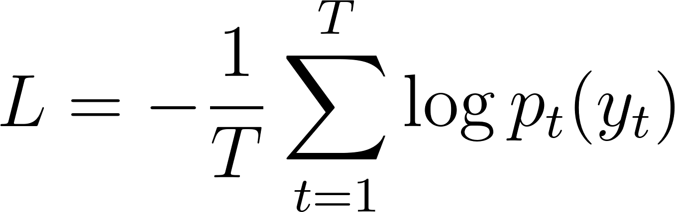
The code implements exactly that:
1 def loss(ids: Array[Int], targets: Array[Int]): Value =
2   val logits = forward(ids)
3   val terms = logits.zip(targets).map { case (row, t) =>
4     val probs = Value.softmax(row)
5     (probs(t) + Value(1e-9)).log() * Value(-1.0)
6   }
7   terms.reduce(_ + _) / Value(terms.size.toDouble)
The small 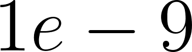 inside the logarithm guards against
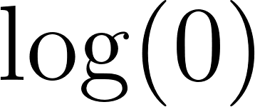 , which is negative infinity. Because every operation here is built from
Value ops, the loss itself is a node in the graph, and calling backward on it produces gradients for all 960 parameters.
One training step zeroes the old gradients, computes the loss, backpropagates, and moves every parameter a small step against its gradient:
1 def trainStep(ids: Array[Int], targets: Array[Int], lr: Double): Double =
2   parameters.foreach(_.grad = 0.0)
3   val l = loss(ids, targets)
4   l.backward()
5   parameters.foreach(p => p.data -= lr * p.grad)
6   l.data
This is stochastic gradient descent: each update uses one window of text rather than the whole corpus. The updates are noisy, but they are cheap and they tend to find good weights quickly. The learning rate lr controls the step size. Too small and training crawls; too large and the loss bounces or diverges.
Gradients must be zeroed before each backward pass because the engine accumulates with +=. Without the reset, gradients from previous steps would pile up and the updates would explode.
Greedy Generation
Once trained, the model generates text one character at a time. At each step it feeds the last blockSize tokens, reads the logits at the final position, picks the highest-scoring character, appends it, and repeats:
1 def generate(start: Array[Int], n: Int, stoi: Map[Char, Int], itos: Map[Int, Char]): String =
2   var ids = start.toList
3   for _ <- 0 until n do
4     val block = ids.takeRight(blockSize).toArray
5     val logits = forward(block)
6     val next = logits.last.map(_.data).zipWithIndex.maxBy(_._1)._2
7     ids = ids :+ next
8   ids.map(itos).mkString
This is greedy decoding: always take the single most likely character. It is deterministic and simple, but it has a known failure mode. Because the model always commits to its top choice, it can fall into loops, repeating the same phrase forever. Sampling from the distribution instead, or restricting the sample to the top few candidates, usually produces more varied text. That is an exercise at the end of the chapter.
The Demo and Its Output
The demo in Main.scala ties everything together. It reads the corpus, builds the vocabulary, trains for three passes over the sliding windows at a learning rate of  , then prints a 60-character sample from the seed
hello :
 1 //> using scala 3.6.4
 2 // Copyright 2026 Mark Watson. All rights reserved.
 3
 4 package microtransformer
 5
 6 import java.nio.file.{Files, Paths}
 7
 8 // Train on data/corpus.txt over sliding next-char windows, print
 9 // loss per pass, print a greedy sample.
10 @main def microDemo(): Unit =
11   val text = Files.readString(Paths.get("data/corpus.txt")).toLowerCase
12   val chars = text.distinct.sorted
13   val stoi = chars.zipWithIndex.toMap
14   val itos = stoi.map(_.swap)
15   val ids = text.map(stoi).toArray
16   val blockSize = 8
17   val model = MicroGPT(chars.size, blockSize)
18   val starts = (0 until ids.length - blockSize).toArray
19   for epoch <- 1 to 3 do
20     var total = 0.0
21     starts.foreach { at =>
22       total += model.trainStep(
23         ids.slice(at, at + blockSize),
24         ids.slice(at + 1, at + blockSize + 1),
25         0.05
26       )
27     }
28     println(f"epoch $epoch mean loss ${total / starts.size}%.3f")
29   println("\nSample:")
30   println(model.generate("hello ".map(stoi).toArray, 60, stoi, itos))
Run it from the example directory:
1 cd source-code/micro-transformer
2 scala-cli run . --main-class microtransformer.microDemo
The corpus has 338 characters, so the block size of 8 yields 330 windows, and three passes make 990 training steps. On a typical laptop each step takes about 3.6 milliseconds, so the whole run finishes in under four seconds. The output is:
1 epoch 1 mean loss 2.521
2 epoch 2 mean loss 1.907
3 epoch 3 mean loss 1.609
4
5 Sample:
6 hello transtranstranstranstranstranstranstranstranstranstranstrans
The loss numbers are the story. A model that knew nothing would spread its probability evenly over the 24 characters, giving a cross-entropy of  . The first pass already lands at 2.521, well below chance, and each pass lowers it further, ending at 1.609 after only three passes. The model is learning the corpus.
The sample confirms it. Starting from the seed hello , the model emits the letters t, r, a, n, s, spelling a fragment of transformer, a word that appears in the training text. It has learned the character statistics of the corpus from raw counts of next-character co-occurrence, with no dictionary and no rules.
The sample also shows the weakness of greedy decoding. It locks onto trans and repeats it to the end, because after trans the most likely continuation is once again the start of a familiar word. The output is honest for a network this small: it has captured the local rhythm of the text but not the ability to plan a whole sentence. Adding sampling, more layers, and more data are the levers that push it toward coherent text.
Tests That Pin Learning
The tests in TransformerTest.scala guard each layer of the stack, from the derivative of a single multiply to the shape of the model’s output:
 1 //> using scala 3.6.4
 2 // Copyright 2026 Mark Watson. All rights reserved.
 3
 4 package microtransformer
 5
 6 // Offline checks. Run with: scala-cli run . --main-class microtransformer.transformerTest
 7 @main def transformerTest(): Unit =
 8   def close(a: Double, b: Double, tol: Double, label: String): Unit =
 9     assert(math.abs(a - b) <= tol, s"$label: expected $b, got $a")
10
11   // Autograd: z = a*b + a with a=2, b=3 gives dz/da = 4, dz/db = 2.
12   val a = Value(2.0)
13   val b = Value(3.0)
14   val z = a * b + a
15   z.backward()
16   close(a.grad, 4.0, 1e-9, "dz/da")
17   close(b.grad, 2.0, 1e-9, "dz/db")
18
19   // Softmax rows sum to 1 and keep order.
20   val probs = Value.softmax(Seq(Value(1.0), Value(2.0), Value(3.0)))
21   close(probs.map(_.data).sum, 1.0, 1e-9, "softmax sums to 1")
22   assert(probs.map(_.data).sliding(2).forall(p => p(0) < p(1)), "softmax keeps order")
23
24   // Model: forward shape is (block, vocab); loss is finite.
25   val text = "hello world, hello scala, hello there!"
26   val chars = text.distinct.sorted
27   val stoi = chars.zipWithIndex.toMap
28   val itos = stoi.map(_.swap)
29   val ids = text.map(stoi).toArray
30   val model = MicroGPT(chars.size, 6, nEmbd = 8, nHead = 2, hidden = 16, seed = 7)
31   val block = ids.take(6)
32   val logits = model.forward(block)
33   assert(logits.size == 6 && logits.forall(_.size == chars.size), "logit shape")
34   val first = model.loss(block, block.tail :+ block.last).data
35   assert(first.isFinite && first > 0.0, s"loss must be finite positive, got $first")
36
37   // Training lowers the loss on this repetitive text.
38   var last = first
39   for step <- 1 to 25 do
40     last = model.trainStep(block, block.tail :+ block.last, 0.05)
41   assert(last < first, s"loss must fall, first=$first last=$last")
42
43   // Generate returns only vocab chars at the asked length.
44   val sample = model.generate("hello ".map(stoi).toArray, 20, stoi, itos)
45   assert(sample.size == 26 && sample.forall(chars.contains), s"bad sample: $sample")
46
47   println("All transformer tests passed.")
The gradient test checks the engine against calculus done by hand. For  with
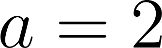 and
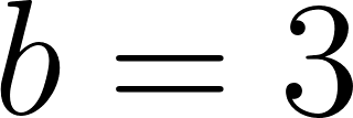 , the derivatives are
 and
 . If the backward closure read the wrong gradient, these numbers would not come out right, and nothing downstream could work.
The softmax test confirms two properties at once: the outputs sum to one, and they preserve the order of their inputs, so a larger logit always yields a larger probability. The shape test verifies that a block of 6 tokens produces 6 rows of vocabSize logits each. The loss test confirms the value is finite and positive, which rules out numerical blowups and .
The most important check is the one that trains for 25 steps and asserts the loss fell. A shape-correct network can still be wired wrong in a way that no structural test catches. Requiring the loss to decrease on a tiny repetitive text is the fastest way to prove that the gradients point downhill and the optimizer follows them. This is the test that most from-scratch implementations skip.
One defect slips past even this test: a parameter that is disconnected from the graph still leaves the loss falling, because the remaining parameters keep learning. The embedding detach described earlier was exactly that case, and the loss fell from 2.597 to 1.804 while the embedding table sat frozen. Catching it requires looking at the gradient itself, which is why the exercises include printing the embedding gradient directly.
Finally, the generation test checks the output length and confirms that every generated character belongs to the vocabulary. Run the suite with:
1 scala-cli run . --main-class microtransformer.transformerTest
A passing run ends with:
1 All transformer tests passed.
Wrap Up
This chapter built a working transformer from the ground up. Starting from a scalar autograd engine, we assembled token embeddings, causal multi-head self-attention, RMSNorm, a residual feed-forward network, and a vocabulary head, then trained it with cross-entropy loss and stochastic gradient descent. Every operation is visible, and every gradient is computed by the same fifty-line engine.
The architecture is not a toy version of a transformer. It is a transformer, with one block and two heads instead of dozens and dozens. Scaling it up means more layers, wider embeddings, more heads, larger vocabularies, and far more data, but the equations and the code shape stay the same. That is the point of building it by hand: the mystery is in the scale, not in the mechanism.
Along the way we fixed a real bug. The embedding lookup originally copied each row into a detached node, which silently cut the embedding table out of the gradient graph. The loss still fell, so the usual training test did not reveal it; only reading the gradients did.
From here, the natural extensions are positional embeddings, so the model knows where tokens sit; sampling with temperature or top-k, so generation stops repeating itself; more layers, so the model can compose features; and a real corpus, so the model has something worth saying.
Optional Practice Problems
Watch the loss fall faster. The demo uses a learning rate of
. Change it to 0.01,0.1, and0.5and record the epoch-3 loss each time. Which rate learns fastest, and at what point does a larger rate start to hurt? Explain the result in terms of the gradient step size.Sample instead of always taking the best. Replace the greedy
maxByingeneratewith a draw from the softmax distribution. Add a temperature that divides the logits before the softmax, so
 sharpens the distribution and
 flattens it. Generate samples at
 , , and
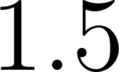 and describe how the repetition changes. Why does a temperature of reproduce greedy decoding?
Give the model a sense of position. Add a learned positional embedding table of shape
 and add row
tto the token embedding at position. Include the new table in parameters, retrain, and compare the loss and sample to the version without it. Does position help on a corpus this repetitive, and why might it matter more on a larger one?Prove the embedding bug for yourself. Temporarily restore the line
var x = ids.map(tokenEmbed(_).map(v => Value(v.data) + Value(0.0))). After onebackwardpass, print the sum of absolute gradients intokenEmbed. Confirm it is zero, then explain in one paragraph why a copy of a number cannot carry a gradient back to its source.Try more heads. Change
nHeadto4and confirm the model still compiles and trains. What constraint mustnHeadsatisfy relative to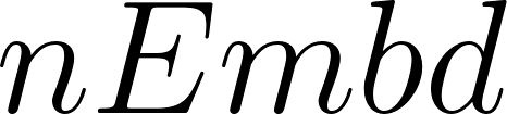 , and why? Then change
nEmbdto and pick a value of
nHeadthat divides it evenly. How does the parameter count change?LayerNorm instead of RMSNorm. Rewrite
rmsNormto subtract the mean before dividing by the standard deviation, the standard LayerNorm. Retrain and compare the final loss. The extra mean subtraction costs a little arithmetic; does it buy anything at this size?Batch the windows. The demo updates the weights after every window. Modify the training loop to process several windows, accumulate their gradients, and apply one averaged update. This is mini-batch gradient descent. Compare the loss curve and the wall-clock time against the per-window version. Why does the batching change the number of parameter updates?
Count the parameters from the shapes. Without running the code, derive the parameter count of 960 from the dimensions in
MicroGPT. Then changehiddento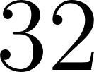 and recompute. Use
model.parameters.sizeto check your arithmetic, and explain which parameter groups grow with the vocabulary and which grow with the embedding width.Break the softmax guard. Remove the max subtraction from
Value.softmax, train on a corpus, and report what happens. Then pass a row of large logits, such as , directly to the unguarded softmax and observe the result. Explain the overflow in terms of and why subtracting a constant does not change the mathematical answer.
Train on your own text. Replace
corpus.txtwith a few hundred characters of your own writing, keeping the same structure. Train the model and inspect the sample. What kinds of mistakes does it make, and do they reflect the letter patterns of your text? This is the smallest possible version of the data problem at the center of language modeling.