Anomaly Detection
Anomaly detection is the process of identifying data points, events, or observations that deviate significantly from the norm. It is widely used in fraud detection, system health monitoring, and medical diagnosis.
In this chapter, we implement a Gaussian Probability Density Function (PDF) anomaly detection algorithm in pure Scala 3 and apply it to the classic Wisconsin Breast Cancer dataset to detect malignant cell samples as anomalies.
All code is in source-code/anomaly-detection.
Why Anomaly Detection, Not Classification
At first glance this looks like a classification problem: sort cell samples into benign and malignant. So why not train a classifier as we did with the neural network? The answer is the shape of the data you usually have. Anomalies are rare and varied. In fraud detection you may see millions of normal transactions and only a handful of frauds, and next month’s fraud may look nothing like last month’s. A supervised classifier needs many labeled examples of every class, and it learns only the kinds of anomalies it has already seen.
Anomaly detection turns the problem around. Instead of learning what an anomaly looks like, it learns what normal looks like, then flags anything that does not fit. We train almost entirely on normal examples, build a model of their distribution, and mark any new point with low probability under that model as an anomaly. This is a form of semi-supervised learning, sometimes called novelty detection: the training set is (mostly) one class, and the model detects departures from it. That is exactly why it suits fraud, intrusion detection, manufacturing defects, and rare-disease screening, where the “normal” class is abundant and the anomalies are few and unpredictable.
How Gaussian Anomaly Detection Works
The Gaussian anomaly detection model assumes that normal features follow a normal (Gaussian) distribution. We train the model using mostly normal (non-anomalous) examples.
- Parameter Estimation: For each feature
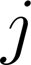 , we compute the mean
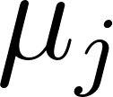 and variance
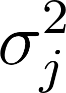 of the training examples:
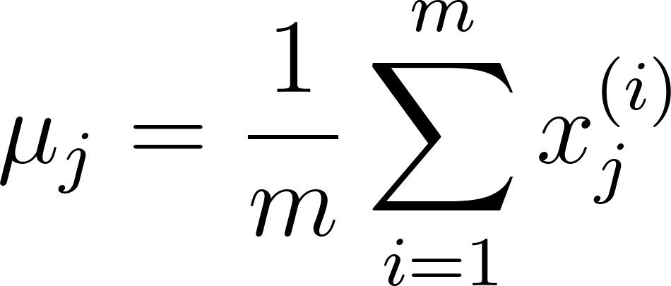
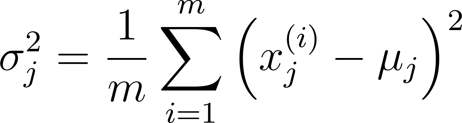
These are not arbitrary formulas. They are the maximum likelihood estimates for a Gaussian: given the training data, they are the mean and variance that make that data most probable under a normal distribution. Note that the variance divides by 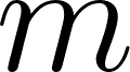 rather than
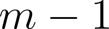 , which is the maximum likelihood form rather than the unbiased sample variance. For a training set of hundreds of examples the difference is negligible.
- Probability Computation: For a new input vector
 , we score each feature with the Gaussian Probability Density Function, which measures how likely that feature value is under the fitted bell curve:
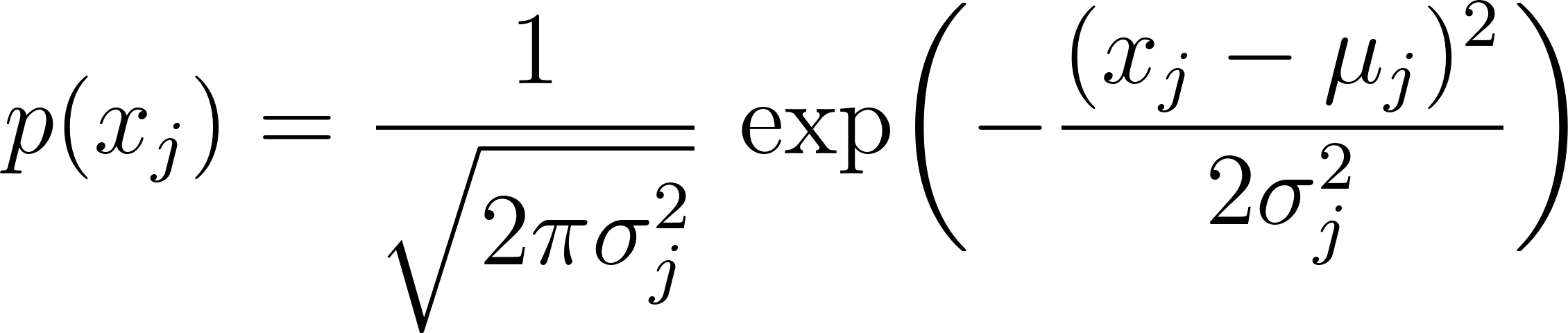
The textbook model then assumes the features are independent and multiplies the per-feature probabilities to get a joint probability 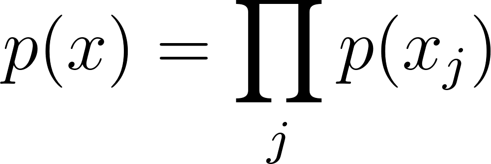 . That independence assumption is rarely true, but the model is robust enough that it works well in practice. Multiplying many probabilities together drives the product toward zero and risks numeric underflow, so our implementation instead averages the per-feature probabilities:
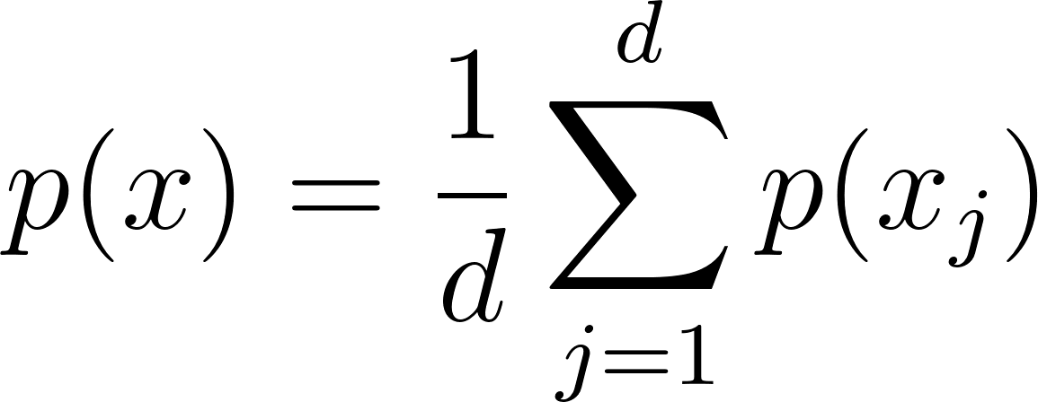
This average is no longer a true joint probability, but it preserves the property we care about: a sample that sits far from the norm on its features gets a low score, and a normal sample gets a high one. It trades theoretical purity for numeric stability, which is a sensible engineering choice for a from-scratch detector.
- Thresholding: We flag an example as an anomaly if its score falls below a threshold parameter
 :
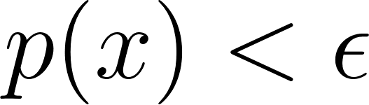
The value of sets the trade-off between catching anomalies and raising false alarms. A high flags more samples (higher recall, more false positives); a low flags fewer (higher precision, more misses). We do not guess it; we tune it, as shown below.
Preprocessing the Data
The model assumes each feature is Gaussian, but real-world data rarely obliges. The Wisconsin features are integer scores from 1 to 10 and are skewed toward the low end, not bell-shaped at all. Feeding skewed data to a Gaussian model weakens it, so we reshape the features first. A logarithmic transform compresses a long right tail and pulls a skewed distribution closer to symmetric, after which min-max scaling maps every feature into 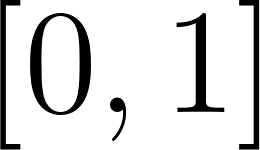 so no single feature dominates the probability by virtue of its raw scale. We do this in anomaly-detection/Main.scala:
 1   val trainingData = (for line <- bufferedSource.getLines() yield
 2     val sarr = line.trim.split(",")
 3     val xs = sarr.take(10).map(_.toDouble)
 4
 5     // Scale features down
 6     for i <- 0 until 9 do xs(i) = xs(i) * 0.1
 7
 8     // Make the data look more like a Gaussian distribution:
 9     var min = 1e6
10     var max = -1e6
11     for i <- 0 until 9 do
12       xs(i) = math.log(xs(i) + 1.2)
13       if xs(i) < min then min = xs(i)
14       if xs(i) > max then max = xs(i)
15
16     val range = max - min
17     for i <- 0 until 9 do
18       xs(i) = if range > 0.0 then (xs(i) - min) / range else 0.0
19
20     xs(9) = (xs(9) - 2.0) * 0.5 // make target output be [0,1] instead of [2,4]
21     xs
22   ).toArray
The dataset is the classic Wisconsin Breast Cancer set from the UCI repository: nine cell-measurement features (clump thickness, cell-size uniformity, and so on) plus an outcome column labeling each sample benign or malignant. The raw outcome uses 2 for benign and 4 for malignant, and the last line remaps it to 0 and 1 so we can treat malignant samples as the anomalies to detect. The small + 1.2 offset inside the logarithm keeps its argument safely positive.
Implementing Anomaly Detection
We encapsulate the model inside the AnomalyDetection class. When the class is instantiated, it splits the dataset into three partitions, and the split is deliberately skewed to match the semi-supervised setup: training keeps almost only normal samples, while cross-validation and testing get a realistic mix of both classes:
 1 class AnomalyDetection(
 2     val numFeatures: Int,
 3     val allExamples: Array[Array[Double]],
 4     seed: Long = 42L
 5 ):
 6   private val outcomeIndex = numFeatures - 1
 7   private val SQRT_2_PI = math.sqrt(2.0 * math.Pi)
 8
 9   // Split datasets (60% training, 28% cross-validation, 12% testing)
10   private val (trainingExamples, crossValidationExamples, testingExamples) =
11     val training = collection.mutable.ArrayBuffer[Array[Double]]()
12     val cv = collection.mutable.ArrayBuffer[Array[Double]]()
13     val test = collection.mutable.ArrayBuffer[Array[Double]]()
14
15     for row <- allExamples do
16       if rng.nextDouble() < 0.6 then
17         // Only keep normal (negative) examples in training, but allow a 10% leak of anomalies
18         if row(outcomeIndex) < 0.5 || rng.nextDouble() < 0.1 then
19           training.append(row)
20       else if rng.nextDouble() < 0.7 then
21         cv.append(row)
22       else
23         test.append(row)
24
25     (training.toArray, cv.toArray, test.toArray)
The three-way split follows standard machine learning methodology, adapted for anomaly detection. The training set estimates  and
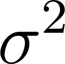 and holds mostly normal data, so the model learns the shape of “normal”. The cross-validation set contains labeled anomalies and is used to tune the one hyperparameter . The test set, untouched during tuning, gives an honest final measure of performance. Keeping tuning and testing separate is what stops us from fooling ourselves: a threshold chosen to look good on the test set would report an optimistic score that new data would not match.
The model estimates and from the training set, then tunes the threshold by scanning a range of values and keeping the one that misclassifies the fewest cross-validation examples:
 1   /** Calculate average feature probability using Gaussian PDF. */
 2   private def p(x: Array[Double]): Double =
 3     var sum = 0.0
 4     // Skip target column at index outcomeIndex
 5     for nf <- 0 until numFeatures - 1 do
 6       val sigma = math.sqrt(sigmaSquared(nf))
 7       val diff = x(nf) - mu(nf)
 8       val exponent = -(diff * diff) / (2.0 * sigmaSquared(nf))
 9       sum += (1.0 / (SQRT_2_PI * sigma)) * math.exp(exponent)
10     sum / numFeatures
11
12   /** Tune epsilon hyperparameter using cross-validation data. */
13   def train(): Unit =
14     // Calculate sigmaSquared from training data using the computed mu values
15     for nf <- 0 until numFeatures - 1 do
16       val sum = trainingExamples.map(x => (x(nf) - mu(nf)) * (x(nf) - mu(nf))).sum
17       sigmaSquared(nf) = sum / numTraining
18
19     var bestErrorCount = Double.MaxValue
20     for epsilonLoop <- 0 to 200 do
21       val epsilon = 0.001 + 0.005 * epsilonLoop
22       val errorCount = evaluateEpsilonOnCV(epsilon)
23       if errorCount <= bestErrorCount then
24         bestErrorCount = errorCount
25         bestEpsilon = epsilon
26
27     println(f"\n**** Best epsilon value = $bestEpsilon%.4f")
28     test(bestEpsilon)
The train method is a simple grid search over : it tries 201 evenly spaced thresholds and keeps whichever one makes the fewest mistakes on the cross-validation data. This brute-force scan is cheap because scoring the CV set is fast, and it avoids any assumption about where the best threshold lies.
Measuring Success: Precision, Recall, and F1
Anomalies are rare, so plain accuracy is a trap. If only 5% of samples are malignant, a lazy detector that calls everything benign scores 95% accuracy while catching zero cancers. We need metrics that focus on the rare positive class. Every prediction falls into one of four cells of a confusion matrix, which the code counts with a clean pattern match:
1       (isTargetAnomaly, isPredictedAnomaly) match
2         case (true, true)   => truePositives += 1
3         case (false, true)  => falsePositives += 1
4         case (true, false)  => falseNegatives += 1
5         case (false, false) => trueNegatives += 1
From these four counts we compute three standard scores. Precision asks: of the samples we flagged, how many were truly anomalies? Recall asks: of the truly anomalous samples, how many did we catch? They pull in opposite directions, so we summarize them with the F1 score, their harmonic mean, which stays low unless both are high:

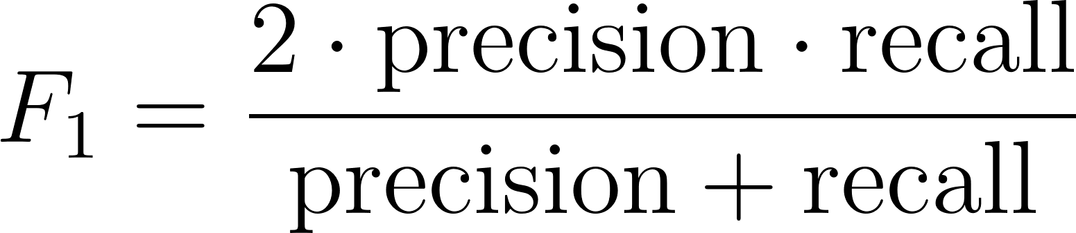
In a medical screen the balance matters: a false negative (missing a cancer) is far worse than a false positive (a needless follow-up test), so in practice you might tune to favor recall. The F1 score gives us a single, honest number to compare against.
Running the Anomaly Detector
When we run the project using scala-cli run ., the main application first displays ASCII histograms of the preprocessed features to confirm their distribution, then splits and trains the detector:
 1 ==================================================
 2 Anomaly Detection: Wisconsin Breast Cancer Data Set
 3 ==================================================
 4
 5 Feature Histograms:
 6
 7 Clump Thickness
 8 0   148 █████████████████████████████
 9 1   79  ███████████████
10 2   144 ████████████████████████████
11 3   118 ███████████████████████
12 4   194 ████████████████████████████████████████
13
14 Uniformity of Cell Size
15 0   374 ████████████████████████████████████████████████████████████████████████████
16 1   66  █████████████
17 2   95  ███████████████████
18 3   81  ████████████████
19 4   67  █████████████
20 ...
21
22 Training anomaly detector on 315 normal samples...
23 Cross-validation samples: 260
24 Testing samples: 108
25
26 **** Best epsilon value = 0.3560
27
28  -- best epsilon = 0.356
29  -- number of test examples = 108
30  -- number of false positives = 5
31  -- number of true positives = 35
32  -- number of false negatives = 4
33  -- number of true negatives = 64
34  -- precision = 0.8750
35  -- recall = 0.8974
36  -- F1 = 0.8861
37
38 Model parameters:
39   best epsilon = 0.3560
40   num features = 10
The confusion matrix in the output tells the full story. Of 108 test samples the detector caught 35 of the 39 malignant cases (recall 0.90) while raising only 5 false alarms among 69 benign cases (precision 0.88). With an F1 score over 88%, the Gaussian PDF anomaly detector successfully identifies malignant cell samples as anomalies based solely on their deviation from normal cell configurations. It never learns what cancer is; it learns what healthy cells look like and reports the samples that do not match.