Leanpub: Publish Early, Publish Often

5. Variation

The variance

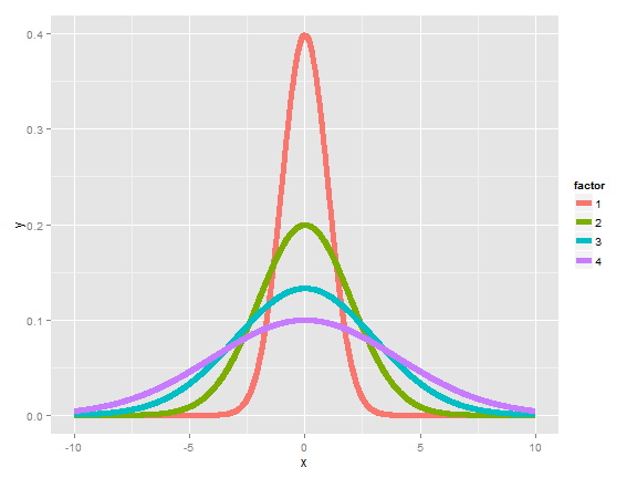
Recall that the mean of distribution was a measure of its center. The variance, on the other hand, is a measure of spread. To get a sense, the plot below shows a series of increasing variances.

We saw another example of how variances changed in the last chapter when we looked at the distribution of averages; they were always centered at the same spot as the original distribution, but are less spread out. Thus, it is less likely for sample means to be far away from the population mean than it is for individual observations. (This is why the sample mean is a better estimate than the population mean.)

If is a random variable with mean $\mu$ , the variance of is defined as

$Var(X) = E[(X - \mu)^2] = E[X^2] - E[X]^2.$

The rightmost equation is the shortcut formula that is almost always used for calculating variances in practice.
Thus the variance is the expected (squared) distance from the mean. Densities with a higher variance are more spread out than densities with a lower variance. The square root of the variance is called the standard deviation. The main benefit of working with standard deviations is that they have the same units as the data, whereas the variance has the units squared.

In this class, we’ll only cover a few basic examples for calculating a variance. Otherwise, we’re going to use the ideas without the formalism. Also remember, what we’re talking about is the population variance. It measures how spread out the population of interest is, unlike the sample variance which measures how spread out the observed data are. Just like the sample mean estimates the population mean, the sample variance will estimate the population variance.

Example

What’s the variance from the result of a toss of a die? First recall that E[X] = 3.5 , as we discussed in the previous lecture. Then let’s calculate the other bit of information that we need, E[X^2] .

$E[X^2] = 1 ^ 2 \times \frac{1}{6} + 2 ^ 2 \times \frac{1}{6} + 3 ^ 2 \times \frac{1}{6} + 4 ^ 2 \times \frac{1}{6} + 5 ^ 2 \times \frac{1}{6} + 6 ^ 2 \times \frac{1}{6} = 15.17$

Thus now we can calculate the variance as:

$Var(X) = E[X^2] - E[X]^2 \approx 2.92.$

Example

What’s the variance from the result of the toss of a (potentially biased) coin with probability of heads (1) of ? First recall that $E[X] = 0 \times (1 - p) + 1 \times p = p.$ Secondly, recall that since is either 0 or 1, X^2 = X . So we know that:

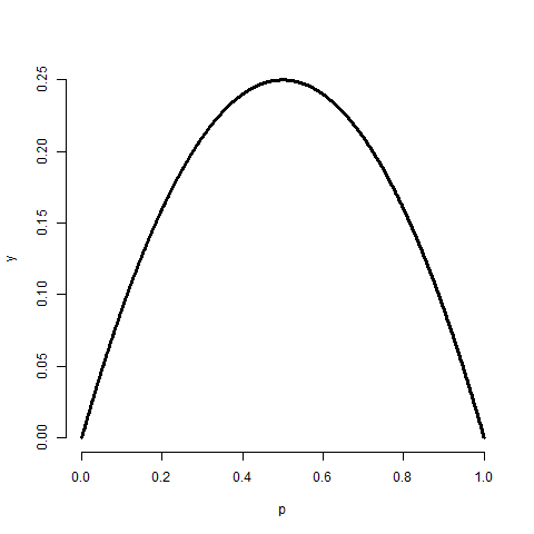
Thus we can now calculate the variance of a coin flip as Var(X) = E[X^2] - E[X]^2 = p - p^2 = p(1 - p). This is a well known formula, so it’s worth committing to memory. It’s interesting to note that this function is maximized at p = 0.5 . The plot below shows this by plotting p(1-p) by .

Plotting the binomial variance

p = seq(0 , 1, length = 1000)
y = p * (1 - p)
plot(p, y, type = "l", lwd = 3, frame = FALSE)

The sample variance

The sample variance is the estimator of the population variance. Recall that the population variance is the expected squared deviation around the population mean. The sample variance is (almost) the average squared deviation of observations around the sample mean. It is given by

$S^2 = \frac{\sum_{i=1} (X_i - \bar X)^2}{n-1}$

The sample standard deviation is the square root of the sample variance. Note again that the sample variance is almost, but not quite, the average squared deviation from the sample mean since we divide by n-1 instead of . Why do we do this you might ask? To answer that question we have to think in the terms of simulations. Remember that the sample variance is a random variable, thus it has a distribution and that distribution has an associated population mean. That mean is the population variance that we’re trying to estimate if we divide by (n-1) rather than .

It is also nice that as we collect more data the distribution of the sample variance gets more concentrated around the population variance that it’s estimating.

Simulation experiments

Watch this video before beginning.

Simulating from a population with variance 1

Let’s try simulating collections of standard normals and taking the variance. If we repeat this over and over, we get a sense of the distribution of sample variances variances.

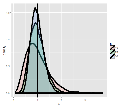
Simulation of variances of samples of standard normals

Notice that these histograms are always centered in the same spot, 1. In other words, the sample variance is an unbiased estimate of the population variances. Notice also that they get more concentrated around the 1 as more data goes into them. Thus, sample variances comprised of more observations are less variable than sample variances comprised of fewer.

Variances of x die rolls

Let’s try the same thing, now only with die rolls instead of simulating standard normals. In this experiment, we simulated samples of die rolls, took the variance and then repeated that process over and over. What is plotted are histograms of the collections of sample variances.

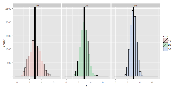
Simulated distributions of variances of dies

Recall that we calculated the variance of a die roll as 2.92 earlier on in this chapter. Notice each of the histograms are centered there. In addition, they get more concentrated around 2.92 as more the variances are comprised of more dice.

The standard error of the mean

At last, we finally get to a perhaps very surprising (and useful) fact: how to estimate the variability of the mean of a sample, when we only get to observe one realization. Recall that the average of random sample from a population is itself a random variable having a distribution, which in simulation settings we can explore by repeated sampling averages. We know that this distribution is centered around the population mean, $E[\bar X] = \mu$ . We also know the variance of the distribution of means of random samples.

The variance of the sample mean is: $Var(\bar X) = \sigma^2 / n$ where $\sigma^2$ is the variance of the population being sampled from.

This is very useful, since we don’t have repeat sample means to get its variance directly using the data. We already know a good estimate of $\sigma^2$ via the sample variance. So, we can get a good estimate of the variability of the mean, even though we only get to observe 1 mean.

Notice also this explains why in all of our simulation experiments the variance of the sample mean kept getting smaller as the sample size increased. This is because of the square root of the sample size in the denominator.

Often we take the square root of the variance of the mean to get the standard deviation of the mean. We call the standard deviation of a statistic its standard error.

Summary notes

The sample variance, , estimates the population variance, $\sigma^2$ .
The distribution of the sample variance is centered around $\sigma^2$ .
The variance of the sample mean is .
- Its logical estimate is .
- The logical estimate of the standard error is $S / \sqrt{n}$ .
, the standard deviation, talks about how variable the population is.
$S/\sqrt{n}$ , the standard error, talks about how variable averages of random samples of size from the population are.

Simulation example 1: standard normals

Watch this video before beginning.

Standard normals have variance 1. Let’s try sampling means of standard normals. If our theory is correct, they should have standard deviation $1/\sqrt{n}$

Simulating means of random normals

> nosim <- 1000
> n <- 10
## simulate nosim averages of 10 standard normals
> sd(apply(matrix(rnorm(nosim * n), nosim), 1, mean))
[1] 0.3156
## Let's check to make sure that this is sigma / sqrt(n)
> 1 / sqrt(n)
[1] 0.3162

So, in this simulation, we simulated 1000 means of 10 standard normals. Our theory says the standard deviation of averages of 10 standard normals must be $1/\sqrt{n}$ . Taking the standard deviation of the 10000 means yields nearly exactly that. (Note that it’s only close, 0.3156 versus 0.31632. To get it to be exact, we’d have to simulate infinitely many means.)

Simulation example 2: uniform density

Standard uniforms have variance 1/12 . Our theory mandates that means of random samples of uniforms have sd $1/\sqrt{12 \times n}$ . Let’s try it with a simulation.

Simulating means of uniforms

> nosim <- 1000
> n <- 10
> sd(apply(matrix(runif(nosim * n), nosim), 1, mean))
[1] 0.09017
> 1 / sqrt(12 * n)
[1] 0.09129

Simulation example 3: Poisson

Poisson(4) random variables have variance . Thus means of random samples of Poisson(4) should have standard deviation $2/\sqrt{n}$ . Again let’s try it out.

Simulating means of Poisson variates

> nosim <- 1000
> n <- 10
> sd(apply(matrix(rpois(nosim * n, 4), nosim), 1, mean))
[1] 0.6219
> 2 / sqrt(n)
[1] 0.6325

Simulation example 4: coin flips

Our last example is an important one. Recall that the variance of a coin flip is p (1 - p) . Therefore the standard deviation of the average of coin flips should be $\sqrt{\frac{p(1-p)}{n}}$ .

Let’s just do the simulation with a fair coin. Such coin flips have variance 0.25. Thus means of random samples of coin flips have sd $1 / (2 \sqrt{n})$ . Let’s try it.

Simulating means of coin flips

> nosim <- 1000
> n <- 10
> sd(apply(matrix(sample(0 : 1, nosim * n, replace = TRUE),
                nosim), 1, mean))
[1] 0.1587
> 1 / (2 * sqrt(n))
[1] 0.1581

Data example

Watch this before beginning.

Now let’s work through a data example to show how the standard error of the mean is used in practice. We’ll use the father.son height data from Francis Galton.

Loading the data

library(UsingR); data(father.son);
x <- father.son$sheight
n<-length(x)

Here’s a histogram of the sons’ heights from the dataset. Let’ calculate different variances and interpret them in this context.

Loading the data

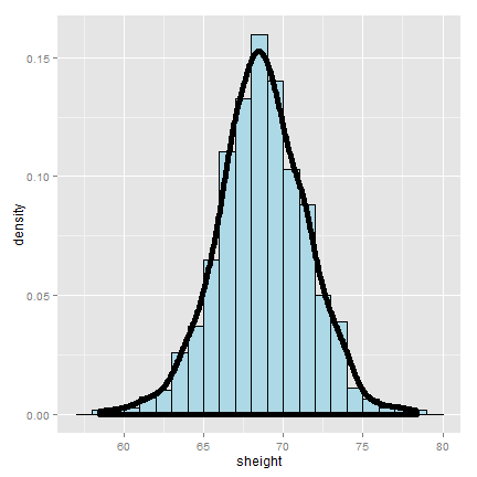
>round(c(var(x), var(x) / n, sd(x), sd(x) / sqrt(n)),2)
[1] 7.92 0.01 2.81 0.09

The first number, 7.92, and its square root, 2.81, are the estimated variance and standard deviation of the sons’ heights. Therefore, 7.92 tells us exactly how variable sons’ heights were in the data and estimates how variable sons’ heights are in the population. In contrast 0.01, and the square root 0.09, estimate how variable averages of sons’ heights are.

Therefore, the smaller numbers discuss the precision of our estimate of the mean of sons’ heights. The larger numbers discuss how variable sons’ heights are in general.

Summary notes

The sample variance estimates the population variance.
The distribution of the sample variance is centered at what its estimating.
It gets more concentrated around the population variance with larger sample sizes.
The variance of the sample mean is the population variance divided by .
- The square root is the standard error.
It turns out that we can say a lot about the distribution of averages from random samples, even though we only get one to look at in a given data set.

Exercises

If I have a random sample from a population, the sample variance is an estimate of?
- The population standard deviation.
- The population variance.
- The sample variance.
- The sample standard deviation.
The distribution of the sample variance of a random sample from a population is centered at what?
- The population variance.
- The population mean.
I keep drawing samples of size from a population with variance $\sigma^2$ and taking their average. I do this thousands of times. If I were to take the variance of the collection of averages, about what would it be?
You get a random sample of observations from a population and take their average. You would like to estimate the variability of averages of $$n$$ observations from this population to better understand how precise of an estimate it is. Do you need to repeated collect averages to do this?
- No, we can multiply our estimate of the population variance by to get a good estimate of the variability of the average.
- Yes, you have to get repeat averages.
A random variable takes the value -4 with probability .2 and 1 with probability .8. What is the variance of this random variable? Watch a video solution to this problem. and look at a version with a worked out solution.
If $\bar X$ and $\bar Y$ are comprised of n iid random variables arising from distributions having means $\mu_x$ and $\mu_y$ , respectively and common variance $\sigma^2$ what is the variance $\bar X - \bar Y$ ? Watch a video solution to this problem here and see a typed up solution here
Let be a random variable having standard deviation $\sigma$ . What can be said about the variance of $X /\sigma$ ? Watch a video solution to this problem here and typed up solutions here.
Consider the following pmf given in R by the code p <- c(.1, .2, .3, .4) and ‘x <- 2 : 5`. What is the variance? Watch a video solution to this problem here and here is the problem worked out.
If you roll ten standard dice, take their average, then repeat this process over and over and construct a histogram, what would be its variance expressed to 3 decimal places? Watch a video solution here and see the text here.