Leanpub: Publish Early, Publish Often

6. Some common distributions

The Bernoulli distribution

The Bernoulli distribution arises as the result of a binary outcome, such as a coin flip. Thus, Bernoulli random variables take (only) the values 1 and 0 with probabilities of (say) and 1-p , respectively. Recall that the PMF for a Bernoulli random variable is $P(X = x) = p^x (1 - p)^{1 - x}$ .

The mean of a Bernoulli random variable is and the variance is p(1 - p) . If we let be a Bernoulli random variable, it is typical to call X=1 as a “success” and X=0 as a “failure”.

If a random variable follows a Bernoulli distribution with success probability we write that $X \sim$ Bernoulli (p) .

Bernoulli random variables are commonly used for modeling any binary trait for a random sample. So, for example, in a random sample whether or not a participant has high blood pressure would be reasonably modeled as Bernoulli.

Binomial trials

The binomial random variables are obtained as the sum of iid Bernoulli trials. So if a Bernoulli trial is the result of a coin flip, a binomial random variable is the total number of heads.

To write it out as mathematics, let $X_1,\ldots,X_n$ be iid Bernoulli (p) , then $X = \sum_{i=1}^n X_i$ is a binomial random variable. We write out that $X \sim$ Binomial (n,p) . The binomial mass function is

$P(X = x) = \left( \begin{array}{c} n \\ x \end{array} \right) p^x(1 - p)^{n-x}$

where $x=0,\ldots,n$ . Recall that the notation

$\left( \begin{array}{c} n \\ x \end{array} \right) = \frac{n!}{x!(n-x)!}$

(read “ choose ”) counts the number of ways of selecting items out of without replacement disregarding the order of the items. It turns out that choose 0 is 1 and choose 1 and choose n-1 are both .

Example

Suppose a friend has 8 children, of which are girls and none are twins. If each gender has an independent % probability for each birth, what’s the probability of getting or more girls out of births?

$\left( \begin{array}{c} 8 \\ 7 \end{array} \right) .5^{7}(1-.5)^{1} + \left( \begin{array}{c} 8 \\ 8 \end{array} \right) .5^{8}(1-.5)^{0} \approx 0.04 .$

Simulating means of coin flips

> choose(8, 7) * 0.5^8 + choose(8, 8) * 0.5^8
[1] 0.03516
> pbinom(6, size = 8, prob = 0.5, lower.tail = FALSE)
[1] 0.03516

The normal distribution

Watch this video before beginning

The normal distribution is easily the handiest distribution in all of statistics. It can be used in an endless variety of settings. Moreover, as we’ll see later on in the course, sample means follow normal distributions for large sample sizes.

Remember the goal of probability modeling. We are assuming a probability distribution for our population as a way of parsimoniously characterizing it. In fact, the normal distribution only requires two numbers to characterize it. Specifically, a random variable is said to follow a normal or Gaussian distribution with mean $\mu$ and variance $\sigma^2$ if the associated density is:

$(2\pi \sigma^2)^{-1/2}e^{-(x - \mu)^2/2\sigma^2}.$

If is a RV with this density then $E[X] = \mu$ and $Var(X) = \sigma^2$ . That is, the normal distribution is characterized by the mean and variance. We write $X\sim N(\mu, \sigma^2)$ to denote a normal random variable. When $\mu = 0$ and $\sigma = 1$ the resulting distribution is called the standard normal distribution. Standard normal RVs are often labeled

Consider an example, if we say that intelligence quotients are normally distributed with a mean of 100 and a standard deviation of 15. Then, we are saying that if we randomly sample a person from this population, the probability that they have an IQ of say 120 or larger, is governed by a normal distribution with a mean of 100 and a variance of 15^2 .

Taken another way, if we know that the population is normally distributed then to estimate everything about the population, we need only estimate the population mean and variance. (Estimated by the sample mean and the sample variance.)

Reference quantiles for the standard normal

The normal distribution is so important that it is useful to memorize reference probabilities and quantiles. The image below shows reference lines at 0, 1, 2 and 3 standard deviations above and below 0. This is for the standard normal; however, all of the rules apply to non standard normals as 0, 1, 2 and 3 standard deviations above and below $\mu$ , the population mean.

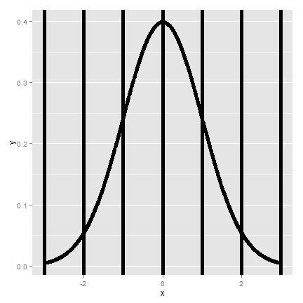
The most relevant probabilities are.

Approximately 68\%, 95\% and 99\% of the normal density lies within 1, 2 and 3 standard deviations from the mean, respectively.
-1.28, -1.645, -1.96 and -2.33 are the $10^{th}$ , $5^{th}$ , $2.5^{th}$ and $1^{st}$ percentiles of the standard normal distribution, respectively.
By symmetry, 1.28, 1.645, 1.96 and 2.33 are the $90^{th}$ , $95^{th}$ , $97.5^{th}$ and $99^{th}$ percentiles of the standard normal distribution, respectively.

Shifting and scaling normals

Since the normal distribution is characterized by only the mean and variance, which are a shift and a scale, we can transform normal random variables to be standard normals and vice versa. For example If $X \sim N(\mu,\sigma^2)$ then:

$Z = \frac{X -\mu}{\sigma} \sim N(0, 1).$

If is standard normal

$X = \mu + \sigma Z \sim N(\mu, \sigma^2)$

then is $X \sim N(\mu,\sigma^2)$ . We can use these facts to answer questions about non-standard normals by relating them back to the standard normal.

Example

What is the $95^{th}$ percentile of a $N(\mu, \sigma^2)$ distribution? Quick answer in R qnorm(.95, mean = mu, sd = sigma). Alternatively, because we have the standard normal quantiles memorized, and we know that 1.645 is its 95th percentile, the answer has to be $\mu + \sigma 1.645$ .

In general, $\mu + \sigma z_0$ where z_0 is the appropriate standard normal quantile.

To put some context on our previous setting, population mean BMI for men is reported as 29 kg/mg^2 with a standard deviation of 4.73. Assuming normality of BMI, what is the population $95^{th}$ percentile? The answer is then:

$29 + 4.73 \times 1.645 = 36.78.$

Or alternatively, we could simply type r qnorm(.95, 29, 4.73) in R.

Now let’s reverse the process. Imaging asking what’s the probability that a randomly drawn subject from this population has a BMI less than 24.27? Notice that

$\frac{24.27 - 29}{4.73} = -1.$

Therefore, 24.27 is 1 standard deviation below the mean. We know that 16% lies below or above 1 standard deviation from the mean. Thus 16% lies below. Alternatively, pnorm(24.27, 29, 4.73) yields the result.

Example

Assume that the number of daily ad clicks for a company is (approximately) normally distributed with a mean of 1020 and a standard deviation of 50. What’s the probability of getting more than 1,160 clicks in a day? Notice that:

$\frac{1160 - 1020}{50} = 2.8$

Therefore, 1,160 is 2.8 standard deviations above the mean. We know from our standard normal quantiles that the probability of being larger than 2 standard deviation is 2.5% and 3 standard deviations is far in the tail. Therefore, we know that the probability has to be smaller than 2.5% and should be very small. We can obtain it exactly as r pnorm(1160, 1020, 50, lower.tail = FALSE) which is 0.3%. Note that we can also obtain the probability as r pnorm(2.8, lower.tail = FALSE).

Example

Consider the previous example again. What number of daily ad clicks would represent the one where 75% of days have fewer clicks (assuming days are independent and identically distributed)? We can obtain this as:

Finding a normal quantile

> qnorm(0.75, mean = 1020, sd = 50)
[1] 1054

The Poisson distribution

Watch this video before beginning.

The Poisson distribution is used to model counts. It is perhaps only second to the normal distribution usefulness. In fact, the Bernoulli, binomial and multinomial distributions can all be modeled by clever uses of the Poisson.

The Poisson distribution is especially useful for modeling unbounded counts or counts per unit of time (rates). Like the number of clicks on advertisements, or the number of people who show up at a bus stop. (While these are in principle bounded, it would be hard to actually put an upper limit on it.) There is also a deep connection between the Poisson distribution and popular models for so-called event-time data. In addition, the Poisson distribution is the default model for so-called contingency table data, which is simply tabulations of discrete characteristics. Finally, when is large and is small, the Poisson is an accurate approximation to the binomial distribution.

The Poisson mass function is:

$P(X = x; \lambda) = \frac{\lambda^x e^{-\lambda}}{x!}$

for $x=0,1,\ldots$ . The mean of this distribution is $\lambda$ . The variance of this distribution is also $\lambda$ . Notice that ranges from 0 to $\infty$ . Therefore, the Poisson distribution is especially useful for modeling unbounded counts.

Rates and Poisson random variables

The Poisson distribution is useful for rates, counts that occur over units of time. Specifically, if $X \sim Poisson(\lambda t)$ where $\lambda = E[X / t]$ is the expected count per unit of time and is the total monitoring time.

Example

The number of people that show up at a bus stop is Poisson with a mean of 2.5 per hour. If watching the bus stop for 4 hours, what is the probability that $3$ or fewer people show up for the whole time?

Finding a normal quantile

> ppois(3, lambda = 2.5 * 4)
[1] 0.01034

Therefore, there is about a 1% chance that 3 or fewer people show up. Notice the multiplication by four in the function argument. Since lambda is specified as events per hour we have to multiply by four to consider the number of events that occur in 4 hours.

Poisson approximation to the binomial

When is large and is small the Poisson distribution is an accurate approximation to the binomial distribution. Formally, if $X \sim \mbox{Binomial}(n, p)$ then is approximately Poisson where $\lambda = n p$ provided that is large is small.

Example, Poisson approximation to the binomial

We flip a coin with success probability 0.01 five hundred times. What’s the probability of 2 or fewer successes?

Finding a normal quantile

> pbinom(2, size = 500, prob = 0.01)
[1] 0.1234
> ppois(2, lambda = 500 * 0.01)
[1] 0.1247

So we can see that the probabilities agree quite well. This approximation is often done as the Poisson model is a more convenient model in many respects.

Exercises

Your friend claims that changing the font to comic sans will result in more ad revenue on your web sites. When presented in random order, 9 pages out of 10 had more revenue when the font was set to comic sans. If it was really a coin flip for these 10 sites, what’s the probability of getting 9 or 10 out of 10 with more revenue for the new font?
A software company is doing an analysis of documentation errors of their products. They sampled their very large codebase in chunks and found that the number of errors per chunk was approximately normally distributed with a mean of 11 errors and a standard deviation of 2. When randomly selecting a chunk from their codebase, whats the probability of fewer than 5 documentation errors?
The number of search entries entered at a web site is Poisson at a rate of 9 searches per minute. The site is monitored for 5 minutes. What is the probability of 40 or fewer searches in that time frame?
Suppose that the number of web hits to a particular site are approximately normally distributed with a mean of 100 hits per day and a standard deviation of 10 hits per day. What’s the probability that a given day has fewer than 93 hits per day expressed as a percentage to the nearest percentage point? Watch a video solution and see the problem.
Suppose that the number of web hits to a particular site are approximately normally distributed with a mean of 100 hits per day and a standard deviation of 10 hits per day. What number of web hits per day represents the number so that only 5% of days have more hits? Watch a video solution and see the problem and solution.
Suppose that the number of web hits to a particular site are approximately normally distributed with a mean of 100 hits per day and a standard deviation of 10 hits per day. Imagine taking a random sample of 50 days. What number of web hits would be the point so that only 5% of averages of 50 days of web traffic have more hits? Watch a video solution and see the problem and solution.
You don’t believe that your friend can discern good wine from cheap. Assuming that you’re right, in a blind test where you randomize 6 paired varieties (Merlot, Chianti, …) of cheap and expensive wines. What is the change that she gets 5 or 6 right? Watch a video solution and see the original problem.
The number of web hits to a site is Poisson with mean 16.5 per day. What is the probability of getting 20 or fewer in 2 days? Watch a video solution and see a written solution.