Leanpub: Publish Early, Publish Often

2. Probability

Probability forms the foundation for almost all treatments of statistical inference. In our treatment, probability is a law that assigns numbers to the long run occurrence of random phenomena after repeated unrelated realizations.

Before we begin discussing probability, let’s dispense with some deep philosophical questions, such as “What is randomness?” and “What is the fundamental interpretation of probability?”. One could spend a lifetime studying these questions (and some have). For our purposes, randomness is any process occurring without apparent deterministic patterns. Thus we will treat many things as if they were random when, in fact they are completely deterministic. In my field, biostatistics, we often model disease outcomes as if they were random when they are the result of many mechanistic components whose aggregate behavior appears random. Probability for us will be the long run proportion of times some occurs in repeated unrelated realizations. So, think of the proportion of times that you get a head when flipping a coin.

For the interested student, I would recommend the books and work by Ian Hacking to learn more about these deep philosophical issues. For us data scientists, the above definitions will work fine.

Where to get a more thorough treatment of probability

In this lecture, we will cover the fundamentals of probability at low enough of a level to have a basic understanding for the rest of the series. For a more complete treatment see the class Mathematical Biostatistics Boot Camp 1, which can be viewed on YouTube here. In addition, there’s the actual Coursera course that I run periodically (this is the first Coursera class that I ever taught). Also there are a set of notes on GitHub. Finally, there’s a follow up class, uninspiringly named Mathematical Biostatistics Boot Camp 2, that is more devoted to biostatistical topics that has an associated YouTube playlist, Coursera Class and GitHub notes.

Kolmogorov’s Three Rules

Watch this lecture before beginning.

Given a random experiment (say rolling a die) a probability measure is a population quantity that summarizes the randomness. The brilliant discovery of the father of probability, the Russian mathematician Kolmogorov, was that to satisfy our intuition about how probability should behave, only three rules were needed.

Consider an experiment with a random outcome. Probability takes a possible outcome from an experiment and:

assigns it a number between 0 and 1
requires that the probability that something occurs is 1
required that the probability of the union of any two sets of outcomes that have nothing in common (mutually exclusive) is the sum of their respective probabilities.

From these simple rules all of the familiar rules of probability can be developed. This all might seem a little odd at first and so we’ll build up our intuition with some simple examples based on coin flipping and die rolling.

I would like to reiterate the important definition that we wrote out: mutually exclusive. Two events are mutually exclusive if they cannot both simultaneously occur. For example, we cannot simultaneously get a 1 and a 2 on a die. Rule 3 says that since the event of getting a 1 and 2 on a die are mutually exclusive, the probability of getting at least one (the union) is the sum of their probabilities. So if we know that the probability of getting a 1 is 1/6 and the probability of getting a 2 is 1/6, then the probability of getting a 1 or a 2 is 2/6, the sum of the two probabilities since they are mutually exclusive.

Consequences of The Three Rules

Let’s cover some consequences of our three simple rules. Take, for example, the probability that something occurs is 1 minus the probability of the opposite occurring. Let be the event that we get a 1 or a 2 on a rolled die. Then A^c is the opposite, getting a 3, 4, 5 or 6. Since and A^c cannot both simultaneously occur, they are mutually exclusive. So the probability that either or A^c is P(A) + P(A^c) . Notice, that the probability that either occurs is the probability of getting a 1, 2, 3, 4, 5 or 6, or in other words, the probability that something occurs, which is 1 by rule number 2. So we have that 1 = P(A) + P(A^c) or that P(A) = 1 - P(A^c) .

We won’t go through this tedious exercise (since Kolmogorov already did it for us). Instead here’s a list of some of the consequences of Kolmogorov’s rules that are often useful.

The probability that nothing occurs is 0
The probability that something occurs is 1
The probability of something is 1 minus the probability that the opposite occurs
The probability of at least one of two (or more) things that can not simultaneously occur (mutually exclusive) is the sum of their respective probabilities
For any two events the probability that at least one occurs is the sum of their probabilities minus their intersection.

This last rules states that $P(A \cup B) = P(A) + P(B) - P(A \cap B)$ shows what is the issue with adding probabilities that are not mutually exclusive. If we do this, we’ve added the probability that both occur in twice! (Watch the video where I draw a Venn diagram to illustrate this).

Example of Implementing Probability Calculus

The National Sleep Foundation (www.sleepfoundation.org) reports that around 3% of the American population has sleep apnea. They also report that around 10% of the North American and European population has restless leg syndrome. Does this imply that 13% of people will have at least one sleep problems of these sorts? In other words, can we simply add these two probabilities?

Answer: No, the events can simultaneously occur and so are not mutually exclusive. To elaborate let:

$\begin{eqnarray*} A_1 & = & \{\mbox{Person has sleep apnea}\} \\ A_2 & = & \{\mbox{Person has RLS}\} \end{eqnarray*}$

Then

$\begin{eqnarray*} P(A_1 \cup A_2 ) & = & P(A_1) + P(A_2) - P(A_1 \cap A_2) \\ & = & 0.13 - \mbox{Probability of having both} \end{eqnarray*}$

Given the scenario, it’s likely that some fraction of the population has both. This example serves as a reminder don’t add probabilities unless the events are mutually exclusive. We’ll have a similar rule for multiplying probabilities and independence.

Random variables

Watch this video before reading this section

Probability calculus is useful for understanding the rules that probabilities must follow. However, we need ways to model and think about probabilities for numeric outcomes of experiments (broadly defined). Densities and mass functions for random variables are the best starting point for this. You’ve already heard of a density since you’ve heard of the famous “bell curve”, or Gaussian density. In this section you’ll learn exactly what the bell curve is and how to work with it.

Remember, everything we’re talking about up to at this point is a population quantity, not a statement about what occurs in our data. Think about the fact that 50% probability for head is a statement about the coin and how we’re flipping it, not a statement about the percentage of heads we obtained in a particular set of flips. This is an important distinction that we will emphasize over and over in this course. Statistical inference is about describing populations using data. Probability density functions are a way to mathematically characterize the population. In this course, we’ll assume that our sample is a random draw from the population.

So our definition is that a random variable is a numerical outcome of an experiment. The random variables that we study will come in two varieties, discrete or continuous. Discrete random variables are random variables that take on only a countable number of possibilities. Mass functions will assign probabilities that they take specific values. Continuous random variable can conceptually take any value on the real line or some subset of the real line and we talk about the probability that they lie within some range. Densities will characterize these probabilities.

Let’s consider some examples of measurements that could be considered random variables. First, familiar gambling experiments like the tossing of a coin and the rolling of a die produce random variables. For the coin, we typically code a tail as a 0 and a head as a 1. (For the die, the number facing up would be the random variable.) We will use these examples a lot to help us build intuition. However, they aren’t interesting in the sense of seeming very contrived. Nonetheless, the coin example is particularly useful since many of the experiments we consider will be modeled as if tossing a biased coin. Modeling any binary characteristic from a random sample of a population can be thought of as a coin toss, with the random sampling performing the roll of the toss and the population percentage of individuals with the characteristic is the probability of a head. Consider, for example, logging whether or not subjects were hypertensive in a random sample. Each subject’s outcome can be modeled as a coin toss. In a similar sense the die roll serves as our model for phenomena with more than one level, such as hair color or rating scales.

Consider also the random variable of the number of web hits for a site each day. This variable is a count, but is largely unbounded (or at least we couldn’t put a specific reasonable upper limit). Random variables like this are often modeled with the so called Poisson distribution.

Finally, consider some continuous random variables. Think of things like lengths or weights. It is mathematically convenient to model these as if they were continuous (even if measurements were truncated liberally). In fact, even discrete random variables with lots of levels are often treated as continuous for convenience.

For all of these kinds of random variables, we need convenient mathematical functions to model the probabilities of collections of realizations. These functions, called mass functions and densities, take possible values of the random variables, and assign the associated probabilities. These entities describe the population of interest. So, consider the most famous density, the normal distribution. Saying that body mass indices follow a normal distribution is a statement about the population of interest. The goal is to use our data to figure out things about that normal distribution, where it’s centered, how spread out it is and even whether our assumption of normality is warranted!

Probability mass functions

A probability mass function evaluated at a value corresponds to the probability that a random variable takes that value. To be a valid pmf a function, , must satisfy:

It must always be larger than or equal to 0.
The sum of the possible values that the random variable can take has to add up to one.

Example

Let be the result of a coin flip where X=0 represents tails and X = 1 represents heads. $p(x) = (1/2)^{x} (1/2)^{1-x}$ for x = 0,1 . Suppose that we do not know whether or not the coin is fair; Let $\theta$ be the probability of a head expressed as a proportion (between 0 and 1). $p(x) = \theta^{x} (1 - \theta)^{1-x}$ for x = 0,1

Probability density functions

Watch this video before beginning.

A probability density function (pdf), is a function associated with a continuous random variable. Because of the peculiarities of treating measurements as having been recorded to infinite decimal expansions, we need a different set of rules. This leads us to the central dogma of probability density functions:

Areas under PDFs correspond to probabilities for that random variable

Therefore, when one says that intelligence quotients (IQ) in population follows a bell curve, they are saying that the probability of a randomly selected person from this population having an IQ between two values is given by the area under the bell curve.

Not every function can be a valid probability density function. For example, if the function dips below zero, then we could have negative probabilities. If the function contains too much area underneath it, we could have probabilities larger than one. The following two rules tell us when a function is a valid probability density function.

Specifically, to be a valid pdf, a function must satisfy

It must be larger than or equal to zero everywhere.
The total area under it must be one.

Example

Suppose that the proportion of help calls that get addressed in a random day by a help line is given by f(x) = 2 x for 0< x < 1 . The R code for plotting this density is

Code for plotting the density

x <- c(-0.5, 0, 1, 1, 1.5)
y <- c(0, 0, 2, 0, 0)
plot(x, y, lwd = 3,frame = FALSE, type = "l")

The result of the code is given below.

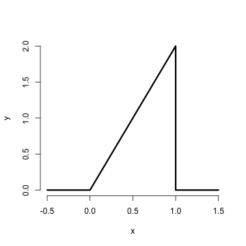
Is this a mathematically valid density? To answer this we need to make sure it satisfies our two conditions. First it’s clearly nonnegative (it’s at or above the horizontal axis everywhere). The area is similarly easy. Being a right triangle in the only section of the density that is above zero, we can calculate it as 1/2 the area of the base times the height. This is $\frac{1}{2} \times 1 \times 2 = 1$

Now consider answering the following question. What is the probability that 75% or fewer of calls get addressed? Remember, for continuous random variables, probabilities are represented by areas underneath the density function. So, we want the area from 0.75 and below, as illustrated by the figure below.

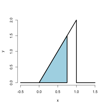
This again is a right triangle, with length of the base as 0.75 and height 1.5. The R code below shows the calculation.

> 1.5 * 0.75/2

[1] 0.5625

Thus, the probability of 75% or fewer calls getting addressed in a random day for this help line is 56%. We’ll do this a lot throughout this class and work with more useful densities. It should be noted that this specific density is a special case of the so called beta density. Below I show how to use R’s built in evaluation function for the beta density to get the probability.

> pbeta(0.75, 2, 1)

[1] 0.5625

Notice the syntax pbeta. In R, a prefix of p returns probabilities, d returns the density, q returns the quantile and r returns generated random variables. (You’ll learn what each of these does in subsequent sections.)

CDF and survival function

Certain areas of PDFs and PMFs are so useful, we give them names. The cumulative distribution function (CDF) of a random variable, , returns the probability that the random variable is less than or equal to the value . Notice the (slightly annoying) convention that we use an upper case to denote a random, unrealized, version of the random variable and a lowercase to denote a specific number that we plug into. (This notation, as odd as it may seem, dates back to Fisher and isn’t going anywhere, so you might as well get used to it. Uppercase for unrealized random variables and lowercase as placeholders for numbers to plug into.) So we could write the following to describe the distribution function :

$F(x) = P(X \leq x)$

This definition applies regardless of
whether the random variable is discrete or continuous. The survival function of a random variable is defined as the probability that the random variable is greater than the value .

Notice that S(x) = 1 - F(x) , since the survival function evaluated at a particular value of is calculating the probability of the opposite event (greater than as opposed to less than or equal to). The survival function is often preferred in biostatistical applications while the distribution function is more generally used (though both convey the same information.)

Example

What are the survival function and CDF from the density considered before?

$F(x) = P(X \leq x) = \frac{1}{2} Base \times Height = \frac{1}{2} (x) \times (2 x) = x^2,$

for $1 \geq x \geq 0$ . Notice that calculating the survival function is now trivial given that we’ve already calculated the distribution function.

Again, R has a function that calculates the distribution function for us in this case, pbeta. Let’s try calculating F(.4) , F(.5) and F(.6)

> pbeta(c(0.4, 0.5, 0.6), 2, 1)

[1] 0.16 0.25 0.36

Notice, of course, these are simply the numbers squared. By default the prefix p in front of a density in R gives the distribution function (pbeta, pnorm, pgamma). If you want the survival function values, you could always subtract by one, or give the argument lower.tail = FALSE as an argument to the function, which asks R to calculate the upper area instead of the lower.

Quantiles

You’ve heard of sample quantiles. If you were the 95th percentile on an exam, you know that 95% of people scored worse than you and 5% scored better. These are sample quantities. But you might have wondered, what are my sample quantiles estimating? In fact, they are estimating the population quantiles. Here we define these population analogs.

The $\alpha^{th}$ quantile of a distribution with distribution function is the point $x_\alpha$ so that

$F(x_\alpha) = \alpha$

So the 0.95 quantile of a distribution is the point so that 95% of the mass of the density lies below it. Or, in other words, the point so that the probability of getting a randomly sampled point below it is 0.95. This is analogous to the sample quantiles where the 0.95 sample quantile is the value so that 95% of the data lies below it.

A percentile is simply a quantile with $\alpha$ expressed as a percent rather than a proportion. The (population) median is the $50^{th}$ percentile. Remember that percentiles are not probabilities! Remember that quantiles have units. So the population median height is the height (in inches say) so that the probability that a randomly selected person from the population is shorter is 50%. The sample, or empirical, median would be the height so in a sample so that 50% of the people in the sample were shorter.

Example

What is the median of the distribution that we were working with before? We want to solve 0.5 = F(x) = x^2 , resulting in the solution

> sqrt(0.5)

[1] 0.7071

Therefore, 0.7071 of calls being answered on a random day is the median. Or, the probability that 70% or fewer calls get answered is 50%.

R can approximate quantiles for you for common distributions with the prefix q in front of the distribution name

> qbeta(0.5, 2, 1)

[1] 0.7071

Exercises

Can you add the probabilities of any two events to get the probability of at least one occurring?
I define a PMF, so that for and we have and . Is this a valid PMF?
What is the probability that 75% or fewer calls get answered in a randomly sampled day from the population distribution from this chapter?
The 97.5th percentile of a distribution is?
Consider influenza epidemics for two parent heterosexual families. Suppose that the probability is 15% that at least one of the parents has contracted the disease. The probability that the father has contracted influenza is 10% while that the mother contracted the disease is 9%. What is the probability that both contracted influenza expressed as a whole number percentage? Watch a video solution to this problem. and see a written out solution.
A random variable, , is uniform, a box from 0 to 1 of height 1. (So that it’s density is for $0\leq x \leq 1$ .) What is it’s median expressed to two decimal places? Watch a video solution to this problem here and see written solutions here.
If a continuous density that never touches the horizontal axis is symmetric about zero, can we say that its associated median is zero? Watch a worked out solution to this problem here and see the question and a typed up answer here