11. Power
Power
Watch this video before beginning. and then watch this video as well.
Power is the probability of rejecting the null hypothesis when it is false.
Ergo, power (as its name would suggest) is a good thing; you want more power.
A type II error (a bad thing, as its name would suggest) is failing to reject
the null hypothesis when it’s false; the probability of a type II error is
usually called  . Note Power
  .
.
Let’s go through an example of calculating power.
Consider our previous example involving RDI.
 versus
  .
Then power is:
.
Then power is:

Note that this is a function that depends on the specific value of  !
Further notice that as
!
Further notice that as  approaches 30 the power approaches
  .
.
Pushing this example further, we reject if

Or, equivalently, if

But, note that, under  .
However, under
.
However, under  .
.
So for this test we could calculate power with this R code:
= 0.05
z = qnorm(1 - alpha)
pnorm(mu0 + z * sigma/sqrt(n), mean = mua, sd = sigma/sqrt(n), lower.tail = FALS\
E)
Let’s plug in the specific numbers for our example where:
 ,
,  ,
,  ,
,  .
.
> mu0 = 30
> mua = 32
> sigma = 4
> n = 16
> z = qnorm(1 - alpha)
> pnorm(mu0 + z * sigma/sqrt(n), mean = mu0, sd = sigma/sqrt(n), lower.tail = FA\
LSE)
[1] 0.05
> pnorm(mu0 + z * sigma/sqrt(n), mean = mua, sd = sigma/sqrt(n), lower.tail = FA\
LSE)
[1] 0.6388
When we plug in  , the value under the null hypothesis, we
get that the probability of rejection is 5%, as the test was designed. However,
when we plug in a value of 32, we get 64%. Therefore, the probability of
rejection is 64% when the true value of
, the value under the null hypothesis, we
get that the probability of rejection is 5%, as the test was designed. However,
when we plug in a value of 32, we get 64%. Therefore, the probability of
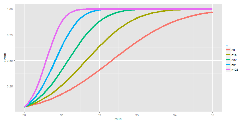
rejection is 64% when the true value of  is 32. We could create
a curve of the power as a function of
is 32. We could create
a curve of the power as a function of  , as seen below.
We also varied the sample size to see how the curve depends on that.
, as seen below.
We also varied the sample size to see how the curve depends on that.
 varies.
The code below shows how to use manipulate to investigate power as the various inputs change.
library(manipulate)
mu0 = 30
myplot <- function(sigma, mua, n, alpha) {
    g = ggplot(data.frame(mu = c(27, 36)), aes(x = mu))
    g = g + stat_function(fun = dnorm, geom = "line", args = list(mean = mu0,
        sd = sigma/sqrt(n)), size = 2, col = "red")
    g = g + stat_function(fun = dnorm, geom = "line", args = list(mean = mua,
        sd = sigma/sqrt(n)), size = 2, col = "blue")
    xitc = mu0 + qnorm(1 - alpha) * sigma/sqrt(n)
    g = g + geom_vline(xintercept = xitc, size = 3)
    g
}
manipulate(myplot(sigma, mua, n, alpha), sigma = slider(1, 10, step = 1, initial\
 = 4),
    mua = slider(30, 35, step = 1, initial = 32), n = slider(1, 50, step = 1,
        initial = 16), alpha = slider(0.01, 0.1, step = 0.01, initial = 0.05))
Question
Watch this video before beginning.
When testing  , notice if power is
  , then

where  . The
unknowns in the equation are:
. The
unknowns in the equation are:  ,
,  ,
,  ,
,
 and the knowns are:
  ,
,  .
Specify any 3 of the unknowns and you can solve for the remainder.
.
Specify any 3 of the unknowns and you can solve for the remainder.
Notes
- The calculation for
 is similar
 - For
 calculate the one sided power using
 (this is only approximately right, it excludes the probability of
getting a large TS in the opposite direction of the truth)
(this is only approximately right, it excludes the probability of
getting a large TS in the opposite direction of the truth) - Power goes up as
 gets larger
 - Power of a one sided test is greater than the power of the associated two sided test
- Power goes up as
 gets further away from $\mu_0$
 - Power goes up as
 goes up
 - Power doesn’t need
 ,
,  and
and  , instead only
- The quantity
 is called the effect size, the difference in the means in standard deviation units.
 - Being unit free, it has some hope of interpretability across settings.
- The quantity
T-test power
Consider calculating power for a Gosset’s t test for our example where
we now assume that  . The power is

Calculating this requires the so-called non-central t distribution.
However, fortunately for us, the R function power.t.test does this very well.
Omit (exactly) any one of the arguments and it solves for it. Our t-test
power again only relies on the effect size.
Let’s do our example trying different options.
# omitting the power and getting a power estimate
> power.t.test(n = 16, delta = 2/4, sd = 1, type = "one.sample", alt = "one.side\d")$power
[1] 0.604
# illustrating that it depends only on the effect size, delta/sd
> power.t.test(n = 16, delta = 2, sd = 4, type = "one.sample", alt = "one.sided"\
)$power
[1] 0.604
# same thing again
> power.t.test(n = 16, delta = 100, sd = 200, type = "one.sample", alt = "one.si\ded")$power
[1] 0.604
# specifying the power and getting n
> power.t.test(power = 0.8, delta = 2/4, sd = 1, type = "one.sample", alt = "one\.sided")$n
[1] 26.14
# again illustrating that the effect size is all that matters
power.t.test(power = 0.8, delta = 2, sd = 4, type = "one.sample", alt = "one.sid\ed")$n
[1] 26.14
# again illustrating that the effect size is all that matters
> power.t.test(power = 0.8, delta = 100, sd = 200, type = "one.sample", alt = "o\ne.sided")$n
[1] 26.14
Exercises
- Power is a probability calculation assuming which is true:
- The null hypothesis
- The alternative hypothesis
- Both the null and alternative
- As your sample size gets bigger, all else equal, what do you think would happen to power?
- It would get larger
- It would get smaller
- It would stay the same
- It cannot be determined from the information given
- What happens to power as
 gets further from
  ?
?
- Power decreases
- Power increases
- Power stays the same
- Power oscillates
- In the context of calculating power, the effect size is?
- The null mean divided by the standard deviation
- The alternative mean divided by the standard error
- The difference between the null and alternative means divided by the standard deviation
- The standard error divided by the null mean
- Recall this problem “Suppose that in an AB test, one advertising scheme led to an average of 10 purchases per day for a sample of 100 days, while the other led to 11 purchases per day, also for a sample of 100 days.
Assuming a common standard deviation of 4 purchases per day.” Assuming that 10 purchases per day is a benchmark null value,
that days are iid and that the standard deviation is 4 purchases for day. Suppose that you
plan on sampling 100 days. What would be the power for a one sided 5%
Z mean test that purchases per day
have increased under the alternative of
 purchase per day? Watch a video
solution and see the text.
purchase per day? Watch a video
solution and see the text. - Researchers would like to conduct a study of healthy adults to detect a four year mean brain volume loss of .01 mm3. Assume that the standard deviation of four year volume loss in this population is .04 mm3. What is necessary sample size for the study for a 5% one sided test versus a null hypothesis of no volume loss to achieve 80% power? Watch the video solution and see the text.