Leanpub: Publish Early, Publish Often

4. Expected values

Expected values characterize a distribution. The most useful expected value, the mean, characterizes the center of a density or mass function. Another expected value summary, the variance, characterizes how spread out a density is. Yet another expected value calculation is the skewness, which considers how much a density is pulled toward high or low values.

Remember, in this lecture we are discussing population quantities. It is convenient (and of course by design) that the names for all of the sample analogs estimate the associated population quantity. So, for example, the sample or empirical mean estimates the population mean; the sample variance estimates the population variance and the sample skewness estimates the population skewness.

The population mean for discrete random variables

The expected value or (population) mean of a random variable is the center of its distribution. For discrete random variable with PMF p(x) , it is defined as follows:

$E[X] = \sum_x xp(x).$

where the sum is taken over the possible values of . Where did they get this idea from? It’s taken from the physical idea of the center of mass. Specifically, E[X] represents the center of mass of a collection of locations and weights, $\{x, p(x)\}$ . We can exploit this fact to quickly calculate population means for distributions where the center of mass is obvious.

The sample mean

It is important to contrast the population mean (the estimand) with the sample mean (the estimator). The sample mean estimates the population mean. Not coincidentally, since the population mean is the center of mass of the population distribution, the sample mean is the center of mass of the data. In fact, it’s exactly the same equation:

$\bar X = \sum_{i=1}^n x_i p(x_i),$

where p(x_i) = 1/n .

Example Find the center of mass of the bars

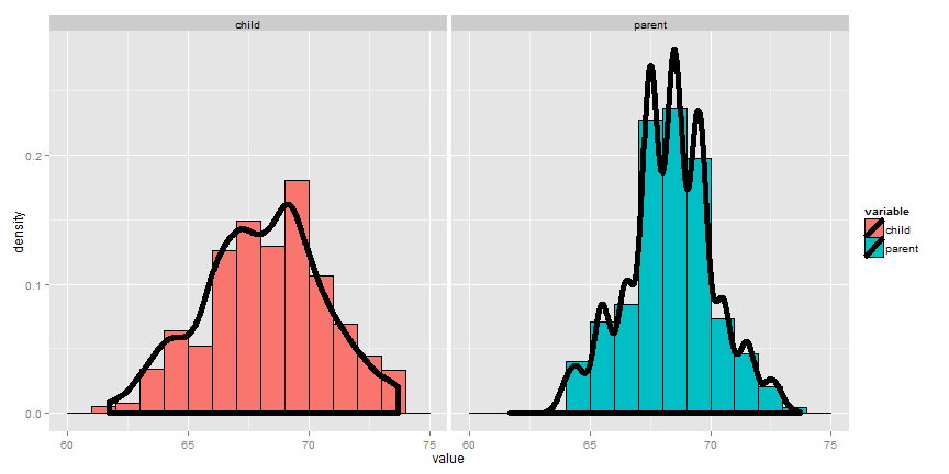
Let’s go through an example of illustrating how the sample mean is the center of mass of observed data. Below we plot Galton’s fathers and sons data:

Loading in and displaying the Galton data

library(UsingR); data(galton); library(ggplot2); library(reshape2)
longGalton <- melt(galton, measure.vars = c("child", "parent"))
g <- ggplot(longGalton, aes(x = value)) + geom_histogram(aes(y = ..density..,  f\
ill = variable), binwidth=1, color = "black") + geom_density(size = 2)
g <- g + facet_grid(. ~ variable)
g

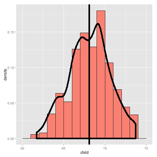
Using rStudio’s manipulate package, you can try moving the histogram around and see what value balances it out. Be sure to watch the video to see this in action.

Using manipulate to explore the mean

library(manipulate)
myHist <- function(mu){
    g <- ggplot(galton, aes(x = child))
    g <- g + geom_histogram(fill = "salmon",
      binwidth=1, aes(y = ..density..), color = "black")
    g <- g + geom_density(size = 2)
    g <- g + geom_vline(xintercept = mu, size = 2)
    mse <- round(mean((galton$child - mu)^2), 3)  
    g <- g + labs(title = paste('mu = ', mu, ' MSE = ', mse))
    g
}
manipulate(myHist(mu), mu = slider(62, 74, step = 0.5))

Going through this exercise, you find that the point that balances out the histogram is the empirical mean. (Note there’s a small distinction here that comes about from rounding with the histogram bar widths, but ignore that for the time being.) If the bars of the histogram are from the observed data, the point that balances it out is the empirical mean; if the bars are the true population probabilities (which we don’t know of course) then the point is the population mean. Let’s now go through some examples of mathematically calculating the population mean.

The center of mass is the empirical mean

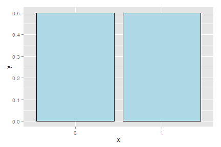
Example of a population mean, a fair coin

Watch the video before beginning here.

Suppose a coin is flipped and is declared 0 or 1 corresponding to a head or a tail, respectively. What is the expected value of ?

$E[X] = .5 \times 0 + .5 \times 1 = .5$

Note, if thought about geometrically, this answer is obvious; if two equal weights are spaced at 0 and 1, the center of mass will be 0.5.

What about a biased coin?

Suppose that a random variable, , is so that P(X=1) = p and P(X=0) = (1 - p) (This is a biased coin when $p\neq 0.5$ .) What is its expected value?

Notice that the expected value isn’t a value that the coin can take in the same way that the sample proportion of heads will also likely be neither 0 nor 1.

This coin example is not exactly trivial as it serves as the basis for a random sample of any population for a binary trait. So, we might model the answer from an election polling question as if it were a coin flip.

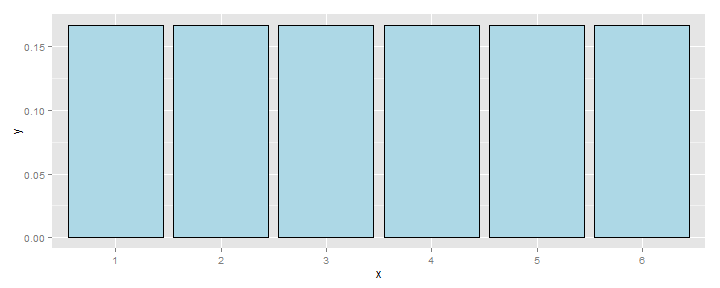
Example Die Roll

Suppose that a die is rolled and is the number face up. What is the expected value of ?

$E[X] = 1 \times \frac{1}{6} + 2 \times \frac{1}{6} + 3 \times \frac{1}{6} + 4 \times \frac{1}{6} + 5 \times \frac{1}{6} + 6 \times \frac{1}{6} = 3.5$

Again, the geometric argument makes this answer obvious without calculation.

Continuous random variables

Watch this video before beginning.

For a continuous random variable, , with density, , the expected value is again exactly the center of mass of the density. Think of it like cutting the continuous density out of a thick piece of wood and trying to find the point where it balances out.

Example

Consider a density where f(x) = 1 for between zero and one. Suppose that follows this density; what is its expected value?

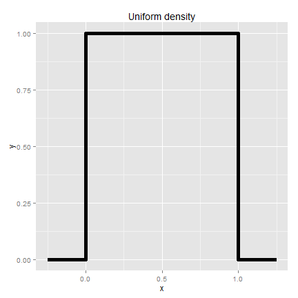
The answer is clear since the density looks like a box, it would balance out exactly in the middle, 0.5.

Facts about expected values

Recall that expected values are properties of population distributions. The expected value, or mean, height is the center of the population density of heights.

Of course, the average of ten randomly sampled people’s height is itself a random variable, in the same way that the average of ten die rolls is itself a random number. Thus, the distribution of heights gives rise to the distribution of averages of ten heights in the same way that distribution associated with a die roll gives rise to the distribution of the average of ten dice.

An important question to ask is: “What does the distribution of averages look like?”. This question is important, since it tells us things about averages, the best way to estimate the population mean, when we only get to observe one average.

Consider the die rolls again. If wanted to know the distribution of averages of 100 die rolls, you could (at least in principle) roll 100 dice, take the average and repeat that process. Imagine, if you could only roll the 100 dice once. Then we would have direct information about the distribution of die rolls (since we have 100 of them), but we wouldn’t have any direct information about the distribution of the average of 100 die rolls, since we only observed one average.

Fortunately, the mathematics tells us about that distribution. Notably, it’s centered at the same spot as the original distribution! Thus, the distribution of the estimator (the sample mean) is centered at the distribution of what it’s estimating (the population mean). When the expected value of an estimator is what its trying to estimate, we say that the estimator is unbiased.

Let’s go through several simulation experiments to see this more fully.

Simulation experiments

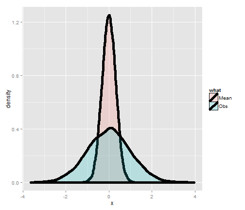
Standard normals

Consider simulating a lot of standard normals and plotting a histogram (the blue density). Now consider simulating lots of averages of 10 standard normals and plotting their histogram (the salmon colored density). Notice that they’re centered in the same spot! It’s also more concentrated around that point. (We’ll discuss that more in the next lectures).

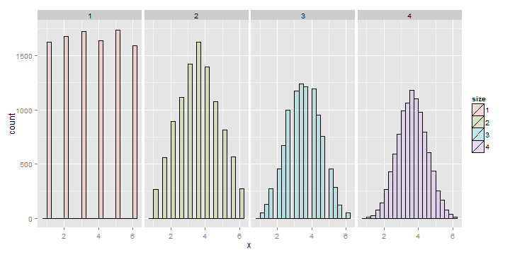
Averages of x die rolls

Consider rolling a die a lot of times and taking a histogram of the results, that’s the left most plot. The bars are equally distributed at the six possible outcomes and thus the histogram is centered around 3.5. Now consider simulating lots of averages of 2 dice. Its histogram is also centered at 3.5. So is it for 3 and 4. Notice also the distribution gets increasing Gaussian looking (like a bell curve) and increasingly concentrated around 3.5.

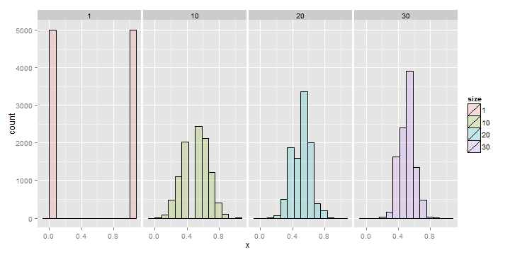
Averages of x coin flips

For the coin flip simulation exactly the same occurs. All of the distributions are centered around 0.5.

Summary notes

Expected values are properties of distributions.
The population mean is the center of mass of population.
The sample mean is the center of mass of the observed data.
The sample mean is an estimate of the population mean.
The sample mean is unbiased: the population mean of its distribution is the mean that it’s trying to estimate.
The more data that goes into the sample mean, the more. concentrated its density / mass function is around the population mean.

Exercises

A standard die takes the values 1, 2, 3, 4, 5, 6 with equal probability. What is the expected value?
Consider a density that is uniform from -1 to 1. (I.e. has height equal to 1/2 and looks like a box starting at -1 and ending at 1). What is the mean of this distribution?
If a population has mean $\mu$ , what is the mean of the distribution of averages of 20 observations from this distribution?
You are playing a game with a friend where you flip a coin and if it comes up heads you give her dollars and if it comes up tails she gives you $Y$ dollars. The odds that the coin is heads is . What is your expected earnings? Watch a video of the solution to this problem and look at the problem and the solution here..
If you roll ten standard dice, take their average, then repeat this process over and over and construct a histogram what would it be centered at? Watch a video solution here and see the original problem here.