8. t Confidence intervals
Small sample confidence intervals
Watch this video before beginning.
In the previous lecture, we discussed creating a confidence interval using the CLT. Our intervals took the form:

In this lecture, we discuss some methods for small samples, notably Gosset’s t distribution and t confidence intervals.
These intervals are of the form:

So the only change is that we’ve replaced the Z quantile now with a t quantile. These are some of the handiest of intervals in all of statistics. If you want a rule between whether to use a t interval or normal interval, just always use the t interval.
Gosset’s t distribution
The t distribution was invented by William Gosset (under the pseudonym “Student”) in 1908. Fisher provided further mathematical details about the distribution later. This distribution has thicker tails than the normal. It’s indexed by a degrees of freedom and it gets more like a standard normal as the degrees of freedom get larger. It assumes that the underlying data are iid Gaussian with the result that

follows Gosset’s t distribution with  degrees of freedom.
(If we replaced
degrees of freedom.
(If we replaced  by
by  the statistic would be exactly
standard normal.)
The interval is
the statistic would be exactly
standard normal.)
The interval is

where  is the relevant quantile from the t distribution.
Code for manipulate
You can use rStudio’s manipulate function to to compare the t and Z distributions.
<- 1000
xvals <- seq(-5, 5, length = k)
myplot <- function(df){
d <- data.frame(y = c(dnorm(xvals), dt(xvals, df)),
x = xvals,
dist = factor(rep(c("Normal", "T"), c(k,k))))
g <- ggplot(d, aes(x = x, y = y))
g <- g + geom_line(size = 2, aes(color = dist))
g
}
manipulate(myplot(mu), mu = slider(1, 20, step = 1))
The difference is perhaps easier to see in the tails. Therefore, the following code plots the upper quantiles of the Z distribution by those of the t distribution.
<- seq(.5, .99, by = .01)
myplot2 <- function(df){
d <- data.frame(n= qnorm(pvals),t=qt(pvals, df),
p = pvals)
g <- ggplot(d, aes(x= n, y = t))
g <- g + geom_abline(size = 2, col = "lightblue")
g <- g + geom_line(size = 2, col = "black")
g <- g + geom_vline(xintercept = qnorm(0.975))
g <- g + geom_hline(yintercept = qt(0.975, df))
g
}
manipulate(myplot2(df), df = slider(1, 20, step = 1))
Summary notes
In this section, we give an overview of important facts about the t distribution.
- The t interval technically assumes that the data are iid normal, though it is robust to this assumption.
- It works well whenever the distribution of the data is roughly symmetric and mound shaped.
- Paired observations are often analyzed using the t interval by taking differences.
- For large degrees of freedom, t quantiles become the same as standard normal quantiles; therefore this interval converges to the same interval as the CLT yielded.
- For skewed distributions, the spirit of the t interval assumptions are violated.
- Also, for skewed distributions, it doesn’t make a lot of sense to center the interval at the mean.
- In this case, consider taking logs or using a different summary like the median.
- For highly discrete data, like binary, other intervals are available.
Example of the t interval, Gosset’s sleep data
Watch this video before beginning.
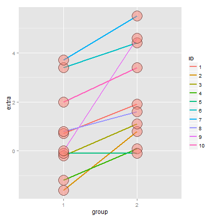
In R typing r data(sleep) brings up the sleep data originally
analyzed in Gosset’s Biometrika paper, which shows the increase in
hours for 10 patients on two soporific drugs. R treats the data as two
groups rather than paired.
The data
> data(sleep)
> head(sleep)
   extra group ID
 1   0.7     1  1
 2  -1.6     1  2
 3  -0.2     1  3
 4  -1.2     1  4
 5  -0.1     1  5
 6   3.4     1  6
Here’s a plot of the data. In this plot paired observations are connected with a line.
Now let’s calculate the t interval for the differences from baseline to follow up. Below we give four different ways for calculating the interval.
<- sleep$extra[1 : 10]; g2 <- sleep$extra[11 : 20]
difference <- g2 - g1
mn <- mean(difference); s <- sd(difference); n <- 10
## Calculating directly
mn + c(-1, 1) * qt(.975, n-1) * s / sqrt(n)
## using R's built in function
t.test(difference)
## using R's built in function, another format
t.test(g2, g1, paired = TRUE)
## using R's built in function, another format
t.test(extra ~ I(relevel(group, 2)), paired = TRUE, data = sleep)
## Below are the results (after a little formatting)
[,1] [,2]
[1,] 0.7001 2.46
[2,] 0.7001 2.46
[3,] 0.7001 2.46
[4,] 0.7001 2.46
Therefore, since our interval doesn’t include 0, our 95% confidence interval estimate for the mean change (follow up - baseline) is 0.70 to 2.45.
Independent group t confidence intervals
Watch this video before beginning.
Suppose that we want to compare the mean blood pressure between two groups in a randomized trial; those who received the treatment to those who received a placebo. The randomization is useful for attempting to balance unobserved covariates that might contaminate our results. Because of the randomization, it would be reasonable to compare the two groups without considering further variables.
We cannot use the paired t interval that we just used for Galton’s data, because the groups are independent. Person 1 from the treated group has no relationship with person 1 from the control group. Moreover, the groups may have different sample sizes, so taking paired differences may not even be possible even if it isn’t advisable in this setting.
We now present methods for creating confidence intervals for comparing independent groups.
Confidence interval
A  confidence interval for the mean difference between the groups,
 is:
is:

The notation  means a t quantile with
 degrees of freedom. The pooled variance estimator is:

This variance estimate is used if one is willing to assume a constant variance across the groups. It is a weighted average of the group-specific variances, with greater weight given to whichever group has the larger sample size.
If there is some doubt about the constant variance assumption, assume a different variance per group, which we will discuss later.
Mistakenly treating the sleep data as grouped
Let’s first go through an example where we treat paired data as if it were independent.
Consider Galton’s sleep data from before. In the code below, we do the R code
for grouped data directly, and using the r t.test function.
<- length(g1); n2 <- length(g2)
sp <- sqrt( ((n1 - 1) * sd(x1)^2 + (n2-1) * sd(x2)^2) / (n1 + n2-2))
md <- mean(g2) - mean(g1)
semd <- sp * sqrt(1 / n1 + 1/n2)
rbind(
md + c(-1, 1) * qt(.975, n1 + n2 - 2) * semd,
t.test(g2, g1, paired = FALSE, var.equal = TRUE)$conf,
t.test(g2, g1, paired = TRUE)$conf
)
The results are:
       [,1]  [,2]
[1,] -0.2039 3.364
[2,] -0.2039 3.364
[3,]  0.7001 2.460
Notice that the paired interval (the last row) is entirely above zero. The grouped interval (first two rows) contains zero. Thus, acknowledging the pairing explains variation that would otherwise be absorbed into the variation for the group means. As a result, treating the groups as independent results in wider intervals. Even if it didn’t result in a shorter interval, the paired interval would be correct as the groups are not statistically independent!
ChickWeight data in R
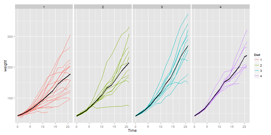
Now let’s try an example with actual independent groups. Load in the ChickWeight
data in R. We are also going to manipulate the dataset to have a total weight gain
variable using dplyr.
library(datasets); data(ChickWeight); library(reshape2)
##define weight gain or loss
wideCW <- dcast(ChickWeight, Diet + Chick ~ Time, value.var = "weight")
names(wideCW)[-(1 : 2)] <- paste("time", names(wideCW)[-(1 : 2)], sep = "")
library(dplyr)
wideCW <- mutate(wideCW,
  gain = time21 - time0
)
Here’s a plot of the data.
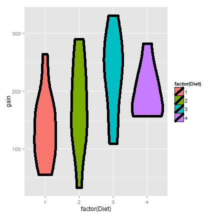
Here’s a plot only of the weight gain for the diets.
Now let’s do a t interval comparing groups 1 and 4. We’ll show the two intervals, one assuming that the variances are equal and one assuming otherwise.
<- subset(wideCW, Diet %in% c(1, 4))
rbind(
t.test(gain ~ Diet, paired = FALSE, var.equal = TRUE, data = wideCW14)$conf,
t.test(gain ~ Diet, paired = FALSE, var.equal = FALSE, data = wideCW14)$conf
)
      [,1]   [,2]
[1,] -108.1 -14.81
[2,] -104.7 -18.30
For the time being, let’s interpret the equal variance interval. Since the interval is entirely below zero it suggest that group 1 had less weight gain than group 4 (at 95% confidence).
Unequal variances
Watch this video before beginning.
Under unequal variances our t interval becomes:

where  is the t quantile calculated with degrees of freedom:

which will be approximately a 95% interval. This works really well.
So when in doubt, just assume unequal variances. Also, we present the formula
for completeness. In practice, it’s easy to mess up, so make sure to do t.test.
Referring back to the previous ChickWeight example, the violin plots suggest that considering
unequal variances would be wise. Recall the code is
> t.test(gain ~ Diet, paired = FALSE, var.equal = FALSE, data = wideCW14)$conf
[2,] -104.7 -18.30
This interval is remains entirely below zero. However, it is wider than the equal variance interval.
Summary notes
- The t distribution is useful for small sample size comparisons.
- It technically assumes normality, but is robust to this assumption within limits.
- The t distribution gives rise to t confidence intervals (and tests, which we will see later)
For other kinds of data, there are preferable small and large sample intervals and tests.
- For binomial data, there’s lots of ways to compare two groups.
- Relative risk, risk difference, odds ratio.
- Chi-squared tests, normal approximations, exact tests.
- For count data, there’s also Chi-squared tests and exact tests.
- We’ll leave the discussions for comparing groups of data for binary and count data until covering glms in the regression class.
- In addition, Mathematical Biostatistics Boot Camp 2 covers many special cases relevant to biostatistics.
Exercises
- For iid Gaussian data, the statistic
 must follow a:
- Z distribution
- t distribution
- Paired differences T confidence intervals are useful when:
- Pairs of observations are linked, such as when there is subject level matching or in a study with baseline and follow up measurements on all participants.
- When there was randomization of a treatment between two independent groups.
- The assumption that the variances are equal for the independent group T interval means that:
- The sample variances have to be nearly identical.
- The population variances are identical, but the sample variances may be different.
- Load the data set
mtcarsin thedatasetsR package. Calculate a 95% confidence interval to the nearest MPG for the variablempg. Watch a video solution and see written solutions. - Suppose that standard deviation of 9 paired differences is $1$. What value would the average difference have to be so that the lower endpoint of a 95% students t confidence interval touches zero? Watch a video solution here and see the text here.
- An independent group Student’s T interval is used instead of
a paired T interval when:
- The observations are paired between the groups.
- The observations between the groups are naturally assumed to be statistically independent.
- As long as you do it correctly, either is fine.
- More details are needed to answer this question. watch a discussion of this problem and see the text.
- Consider the
mtcarsdataset. Construct a 95% T interval for MPG comparing 4 to 6 cylinder cars (subtracting in the order of 4 - 6) assume a constant variance. Watch a video solution and see the text. 10. - If someone put a gun to your head and said “Your confidence interval
must contain what it’s estimating or I’ll pull the trigger”, what would
be the smart thing to do?
- Make your interval as wide as possible.
- Make your interval as small as possible.
- Call the authorities. Watch the video solution and see the text.
- Refer back to comparing MPG for 4 versus 6 cylinders (question 7).
What do you conclude?
- The interval is above zero, suggesting 6 is better than 4 in the terms of MPG.
- The interval is above zero, suggesting 4 is better than 6 in the terms of MPG.
- The interval does not tell you anything about the hypothesis test; you have to do the test.
- The interval contains 0 suggesting no difference. Watch a video solution and see the text.
- Suppose that 18 obese subjects were randomized, 9 each, to a new diet pill and a placebo. Subjects’ body mass indices (BMIs) were measured at a baseline and again after having received the treatment or placebo for four weeks. The average difference from follow-up to the baseline (followup - baseline) was 3 kg/m2 for the treated group and 1 kg/m2 for the placebo group. The corresponding standard deviations of the differences was 1.5 kg/m2 for the treatment group and 1.8 kg/m2 for the placebo group. The study aims to answer whether the change in BMI over the four week period appear to differ between the treated and placebo groups. What is the pooled variance estimate? Watch a video solution here and see the text here.