Reinforcement Learning: Value Iteration and Q-Learning
Reinforcement learning (RL) is the branch of machine learning that studies how an agent should act in an environment in order to maximize a cumulative reward signal. Unlike supervised learning, there is no labeled dataset saying “here is the right action for this input”. Instead the agent must discover, through trial and error, which sequences of actions eventually pay off. This framing captures an enormous range of practical problems: robots learning to walk, programs learning to play board games, recommender systems learning what content to surface, and adaptive controllers for chemical plants, elevators, and datacenter cooling systems.
In this chapter we implement two classical RL algorithms in Gerbil Scheme, both from scratch and with no external dependencies. The first, Value Iteration, solves a fully known Markov Decision Process by directly computing the optimal value of every state. The second, Q-Learning, drops the assumption that the transition model is known and learns action values by simply interacting with an environment. Value Iteration and Q-Learning are the two canonical algorithms in the field, and they illustrate the two very different worlds RL practitioners work in: model-based planning versus model-free learning.
Theoretical Background
Markov Decision Processes
A Markov Decision Process (MDP) is the standard mathematical framework for RL. An MDP consists of:
- A finite set of states
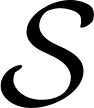 .
.
- A finite set of actions
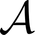 .
.
- A transition function
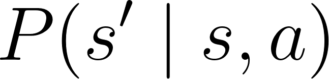 giving the probability of ending in state
 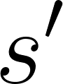 after taking action
  in state
  .
.
- A reward function
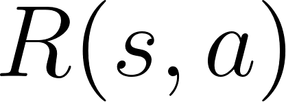 giving the expected immediate reward for taking action in state .
- A discount factor
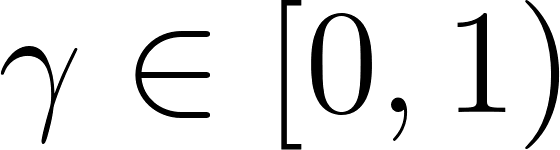 that weighs immediate rewards more heavily than distant ones.
The Markov property is that the next state depends only on the current state and action, not on the history that led to the current state. This assumption is what makes the problem tractable, and it is a surprisingly good approximation in many domains.
A policy  is a rule that tells the agent which action to take in each state. The value of following policy starting in state is the expected discounted return:

The goal of RL is to find the optimal policy 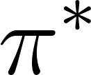 that maximizes this expected return from every state.
The Bellman Optimality Equation
The optimal value function 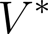 satisfies the recursive Bellman optimality equation:

This equation says: the value of the best action from state equals the immediate reward plus the discounted expected value of where you end up. Once we know , the optimal policy is trivially derived by acting greedily with respect to it:

Value Iteration
Value Iteration solves the Bellman equation by turning it into an update rule. Starting from 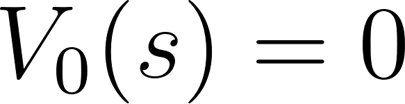 everywhere, we repeatedly apply:

This contraction converges to for any 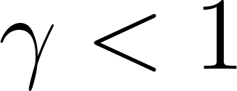 . In practice we stop when the maximum change across all states over one sweep drops below a small threshold.
Value Iteration requires the full transition and reward model of the environment. When we have that model, it is elegant and exact.
Q-Learning
In many real problems we do not know 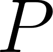 and
and 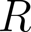 . The agent has to learn purely from experience. This is what Q-Learning does. Instead of storing a value per state, we store a Q-value
 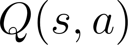 for every state-action pair. Given a transition
 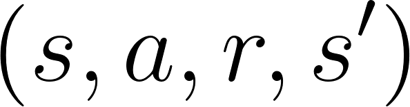 observed during play, we update:

The bracketed quantity is called the temporal-difference (TD) error. It is the discrepancy between our current estimate of and the newly observed one-step lookahead. The learning rate 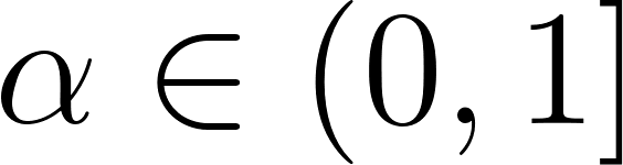 controls how aggressively we pull our estimate toward the new evidence.
Exploration versus Exploitation
If the agent always picks the action it currently thinks is best, it will never discover superior alternatives. To break out of this trap, Q-Learning uses an \epsilon$-greedy strategy: with probability  take a random action (exploration), otherwise take the current best action (exploitation). Over the course of training we anneal from a large value (say 1.0) down to a small floor (say 0.01), so the agent explores aggressively early and exploits its learned knowledge later.
Project Structure
The project directory source_code/reinforcement-learning contains:
| File | Description |
|---|---|
mdp_demo.ss |
Value Iteration on a deterministic 3x3 grid world. |
frozen_lake_qlearning.ss |
Q-Learning on the stochastic 4x4 FrozenLake environment. |
Makefile |
Two targets: run-mdp and run-qlearning. |
gerbil.pkg |
Package declaration. |
Each Scheme file is self-contained: no shared modules, no external data files, and no dependencies beyond Gerbil’s standard library.
Example 1: Value Iteration on a 3×3 Grid World
The first example plants an agent in a 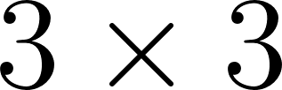 grid with a rewarding goal cell and a punishing trap. The environment is deterministic: attempting to move up in cell 4 always lands in cell 1. Attempting to walk into a wall keeps the agent in place.
Grid Layout
We number the cells row-major from 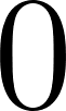 to
to 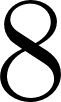 :
:
1 +---+---+---+
2 | 0 | 1 | 2 |
3 +---+---+---+
4 | 3 | 4 | 5 |   <- cell 5 is a trap, R = -5
5 +---+---+---+
6 | 6 | 7 | 8 |   <- cell 8 is the goal, R = +10
7 +---+---+---+
The rewards are attached to actions taken from these cells (rather than to arriving there), so any action from cell 8 pays out +10 and any action from cell 5 pays out -5.
Imports and Formatting Helpers
The file begins with imports and two small helpers for pretty-printing floating-point numbers. Gerbil’s default float printing produces long decimal expansions (like 65.6100000000...), which is inconvenient for reporting value functions:
 1 ;; File: mdp_demo.ss
 2 (import :std/format
 3         :std/pregexp
 4         :gerbil/gambit)
 5
 6 ;; Find index of character in string (helper for format-decimal)
 7 (def (string-index str char)
 8   (let ((len (string-length str)))
 9     (let loop ((i 0))
10       (cond
11         ((= i len) #f)
12         ((char=? (string-ref str i) char) i)
13         (else (loop (+ i 1)))))))
14
15 ;; Format floating point numbers to a fixed number of decimal places
16 (def (format-decimal x places)
17   (let* ((multiplier (expt 10 places))
18          (rounded (/ (round (* x multiplier)) multiplier))
19          (str (number->string rounded)))
20     (let ((dot-pos (string-index str #\.)))
21       (let ((formatted-str
22              (if dot-pos
23                (let* ((frac-len (- (string-length str) dot-pos 1))
24                       (diff (- places frac-len)))
25                  (if (> diff 0)
26                    (string-append str (make-string diff #\0))
27                    str))
28                (string-append str "." (make-string places #\0)))))
29         (if (char=? (string-ref formatted-str 0) #\.)
30           (string-append "0" formatted-str)
31           formatted-str)))))
A 3D Vector Helper
The transition model is naturally represented as a 3-dimensional array indexed by action, source state, and next state. Gerbil vectors are one-dimensional, so we build a 3D vector by nesting:
 1 ;; Multi-dimensional vector creation helper
 2 (def (make-3d-vector d1 d2 d3 (val 0.0))
 3   (let ((v1 (make-vector d1)))
 4     (do ((i 0 (+ i 1)))
 5         ((= i d1) v1)
 6       (let ((v2 (make-vector d2)))
 7         (do ((j 0 (+ j 1)))
 8             ((= j d2))
 9           (vector-set! v2 j (make-vector d3 val)))
10         (vector-set! v1 i v2)))))
Reading a single probability out of then requires three vector-ref calls: (vector-ref (vector-ref (vector-ref P a) s) sp).
The Value Iteration Loop
The core algorithm is a direct translation of the Bellman update. We sweep over every state, compute the value of each action as the immediate reward plus the discounted expected value of successor states, keep the best action, and remember both the new value and the greedy policy:
 1 ;; Value Iteration Algorithm
 2 (def (value-iteration nS nA P R (gamma 0.9) (threshold 1e-6))
 3   (let ((V (make-vector nS 0.0))
 4         (policy (make-vector nS 0))
 5         (iterations 0))
 6     (let loop ()
 7       (set! iterations (+ iterations 1))
 8       (let ((new-V (make-vector nS 0.0))
 9             (max-delta 0.0))
10         (do ((s 0 (+ s 1)))
11             ((= s nS))
12           (let ((best-val -1.0e9)
13                 (best-a 0))
14             (do ((a 0 (+ a 1)))
15                 ((= a nA))
16               (let ((val (vector-ref (vector-ref R s) a)))
17                 (do ((sp 0 (+ sp 1)))
18                     ((= sp nS))
19                   (let ((prob (vector-ref (vector-ref (vector-ref P a) s) sp)))
20                     (set! val (+ val (* gamma prob (vector-ref V sp))))))
21                 (when (> val best-val)
22                   (set! best-val val)
23                   (set! best-a a))))
24             (vector-set! new-V s best-val)
25             (vector-set! policy s best-a)
26             (set! max-delta (max max-delta (abs (- best-val (vector-ref V s)))))))
27         (set! V new-V)
28         (if (< max-delta threshold)
29           `((policy . ,policy)
30             (V . ,V)
31             (iterations . ,iterations))
32           (loop))))))
The termination criterion max-delta < threshold is the numerical realization of “the values have stopped changing”.
Building the Transition and Reward Tables
The main function wires up the grid dynamics. The four actions are UP, RIGHT, DOWN, and LEFT, encoded as ,  ,
,  ,
, 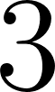 . Given a state we compute its row and column, apply the direction, clip to the grid boundary (bounce), and set the transition probability to 1.0:
 1 (def (main)
 2   (let* ((nS 9)
 3          (nA 4)
 4          ;; transition probability matrix P[nA][nS][nS]
 5          (P (make-3d-vector nA nS nS 0.0))
 6          ;; dirs: UP, RIGHT, DOWN, LEFT
 7          (dirs '#((-1 0) (0 1) (1 0) (0 -1))))
 8
 9     ;; Set up grid transitions
10     (do ((s 0 (+ s 1)))
11         ((= s nS))
12       (let* ((r (quotient s 3))
13              (c (modulo s 3)))
14         (do ((a 0 (+ a 1)))
15             ((= a nA))
16           (let* ((dir (vector-ref dirs a))
17                  (dr (car dir))
18                  (dc (cadr dir))
19                  (nr (+ r dr))
20                  (nc (+ c dc))
21                  (next-s (if (and (>= nr 0) (< nr 3) (>= nc 0) (< nc 3))
22                            (+ (* nr 3) nc)
23                            s)))
24             (vector-set! (vector-ref (vector-ref P a) s) next-s 1.0)))))
The reward matrix is initialized to zero everywhere and then patched: any action from the goal cell 8 gives +10, and any action from the trap cell 5 gives -5:
 1     ;; Set up reward matrix R[nS][nA]
 2     (let ((R (make-vector nS)))
 3       (do ((s 0 (+ s 1)))
 4           ((= s nS))
 5         (vector-set! R s (make-vector nA 0.0)))
 6       ;; Set up specific target rewards
 7       (do ((a 0 (+ a 1)))
 8           ((= a nA))
 9         (vector-set! (vector-ref R 8) a 10.0)
10         (vector-set! (vector-ref R 5) a -5.0))
11
12       ;; Run Value Iteration
13       (let* ((res (value-iteration nS nA P R 0.9))
14              (policy (cdr (assoc 'policy res)))
15              (V (cdr (assoc 'V res)))
16              (iterations (cdr (assoc 'iterations res)))
17              (arrows '#("↑" "→" "↓" "←")))
18         (displayln "=== Custom 3×3 Grid World ===")
19         (displayln "Optimal policy:")
20         (do ((r 0 (+ r 1)))
21             ((= r 3))
22           (let ((line ""))
23             (do ((c 0 (+ c 1)))
24                 ((= c 3))
25               (let* ((idx (+ (* r 3) c))
26                      (a (vector-ref policy idx))
27                      (arrow (vector-ref arrows a)))
28                 (set! line (string-append line "  " arrow "  "))))
29             (displayln line)))
30
31         (displayln "")
32         (display "Value function: [")
33         (do ((s 0 (+ s 1)))
34             ((= s nS))
35           (display (format-decimal (vector-ref V s) 2))
36           (when (< s (- nS 1)) (display ", ")))
37         (displayln "]")
38         (displayln "Iterations: " iterations)))))
39
40 (main)
Running the Value Iteration Demo
Run either make run-mdp or invoke the interpreter directly:
 1 $ make run-mdp
 2 gxi mdp_demo.ss
 3 === Custom 3×3 Grid World ===
 4 Optimal policy:
 5   →    ↓    ↓
 6   →    ↓    ↓
 7   →    →    →
 8
 9 Value function: [65.61, 72.90, 76.50, 72.90, 81.00, 85.00, 81.00, 90.00, 100.00]
10 Iterations: 154
Interpreting the Value Iteration Results
- Optimal policy arrows show the greedy action from every cell. From the top-left corner (cell 0) the best action is RIGHT, which begins the path 0 -> 1 -> 2 -> 5 -> 8. Even though cell 5 is a trap, the policy is willing to accept the -5 penalty once because reaching the goal is worth so much more.
- Value function: cell 8 has value 100.0, which is the goal reward of 10 amplified through the loop where every action from cell 8 collects another +10 discounted by
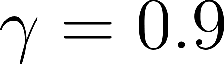 . The infinite geometric series
  sums to exactly
  .
.
- Value monotonicity: values decrease with distance from the goal, from 100.0 at cell 8 down to 65.61 at cell 0. Each step away from the goal multiplies the payoff by
 .
.
- Cell 5 = 85.0: even though cell 5 is a trap, its value is still positive and high, because from cell 5 you can immediately move DOWN into the goal at cell 8. The trap penalty is paid once, but the goal payoff dominates.
- 154 iterations: the algorithm converged in 154 sweeps to a maximum change of less than
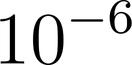 . The convergence rate is governed by : a larger means longer-horizon planning and therefore more iterations before things settle.
Example 2: Q-Learning on FrozenLake
The second example is much more interesting because the agent no longer knows the environment ahead of time and the environment itself is stochastic. FrozenLake is a 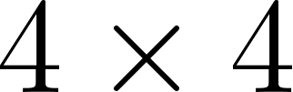 grid modelled after a slippery frozen pond:
1 S F F F
2 F H F H
3 F F F H
4 H F F G
Sis the start (cell 0).Gis the goal (cell 15). Stepping ontoGyields a reward of +1 and ends the episode.Hcells are holes. Stepping intoHends the episode with reward 0.Fare frozen cells that are safe to walk on.
The twist is that the ice is slippery. With probability 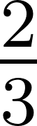 the agent slips and moves in one of the two orthogonal directions instead of the one it chose. This means the agent cannot deterministically follow any path; it has to learn a policy that is robust to slipping.
Building the Environment
The environment holds its state in a Gerbil hash table:
 1 ;; File: frozen_lake_qlearning.ss
 2 (import :std/format
 3         :std/pregexp
 4         :gerbil/gambit)
 5
 6 ;; ... string-index and format-decimal helpers ...
 7
 8 ;; Pad string left
 9 (def (pad-left str len char)
10   (let ((diff (- len (string-length str))))
11     (if (> diff 0)
12       (string-append (make-string diff char) str)
13       str)))
14
15 ;; Environment Setup
16 (def (make-frozen-lake (slippery #t))
17   (let ((state 0)
18         (grid '#("S" "F" "F" "F" "F" "H" "F" "H" "F" "F" "F" "H" "H" "F" "F" "G")))
19     (list->hash-table
20       `((state . ,state)
21         (slippery . ,slippery)
22         (grid . ,grid)
23         (n-states . 16)
24         (n-actions . 4)))))
25
26 (def (frozen-lake-reset! env)
27   (hash-put! env 'state 0)
28   0)
frozen-lake-step! implements the slippery dynamics. If slippery is true, it flips a coin: with probability the requested action is replaced by  or
or  (a
(a 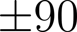 -degree slip). Otherwise the action goes through as intended:
 1 (def (frozen-lake-step! env action)
 2   (let* ((state (hash-ref env 'state))
 3          (slippery (hash-ref env 'slippery))
 4          (grid (hash-ref env 'grid))
 5          ;; If slippery, there's a 2/3 chance of slipping to an orthogonal direction
 6          (a (if (and slippery (< (random-real) 0.667))
 7                 (modulo (+ action (if (< (random-real) 0.5) -1 1) 4) 4)
 8                 action))
 9          (r (quotient state 4))
10          (c (modulo state 4))
11          ;; dirs: UP (0), RIGHT (1), DOWN (2), LEFT (3)
12          (dirs '#((-1 0) (0 1) (1 0) (0 -1)))
13          (dir (vector-ref dirs a))
14          (dr (car dir))
15          (dc (cadr dir))
16          (nr (max 0 (min 3 (+ r dr))))
17          (nc (max 0 (min 3 (+ c dc))))
18          (next-state (+ (* nr 4) nc))
19          (cell (vector-ref grid next-state))
20          (reward (if (equal? cell "G") 1.0 0.0))
21          (done (or (equal? cell "H") (equal? cell "G"))))
22     (hash-put! env 'state next-state)
23     `((next-state . ,next-state)
24       (reward . ,reward)
25       (done . ,done))))
The step function returns an association list with three keys: the new state, the reward received, and a boolean indicating whether the episode is over.
The Q-Table
The Q-table is a vector of vectors: 16 states, each with a 4-element vector of Q-values (one per action). Two small helpers, argmax and vector-max, extract the greedy action and best Q-value for a state:
 1 ;; Q-Table Setup and Helpers
 2 (def (make-q-table states actions)
 3   (let ((Q (make-vector states)))
 4     (do ((i 0 (+ i 1)))
 5         ((= i states) Q)
 6       (vector-set! Q i (make-vector actions 0.0)))))
 7
 8 (def (argmax vec)
 9   (let ((len (vector-length vec)))
10     (let loop ((i 1) (best-idx 0) (best-val (vector-ref vec 0)))
11       (if (= i len)
12         best-idx
13         (let ((val (vector-ref vec i)))
14           (if (> val best-val)
15             (loop (+ i 1) i val)
16             (loop (+ i 1) best-idx best-val)))))))
17
18 (def (vector-max vec)
19   (let ((len (vector-length vec)))
20     (let loop ((i 1) (best-val (vector-ref vec 0)))
21       (if (= i len)
22         best-val
23         (loop (+ i 1) (max best-val (vector-ref vec i)))))))
Evaluating the Current Policy
To measure progress during training we need a way to run the greedy policy that Q currently implies, without any exploration noise, and count how often it reaches the goal. evaluate runs a fixed number of episodes (default 100) using pure argmax action selection and returns the fraction of episodes that ended in success:
 1 ;; Evaluation
 2 (def (evaluate env Q (episodes 100))
 3   (let ((wins 0))
 4     (do ((i 0 (+ i 1)))
 5         ((= i episodes) (/ wins (exact->inexact episodes)))
 6       (frozen-lake-reset! env)
 7       (let loop ((s 0) (steps 0))
 8         (let* ((a (argmax (vector-ref Q s)))
 9                (step-res (frozen-lake-step! env a))
10                (next-state (cdr (assoc 'next-state step-res)))
11                (reward (cdr (assoc 'reward step-res)))
12                (done (cdr (assoc 'done step-res))))
13           (cond
14             ((and done (= reward 1.0))
15              (set! wins (+ wins 1)))
16             ((and (not done) (< steps 100))
17              (loop next-state (+ steps 1)))))))))
Note the 100-step cap. Without it, a very bad or oscillating policy could loop forever on the ice without ever hitting a hole or the goal.
The Q-Learning Training Loop
Here is the heart of the algorithm. For each of 10,000 episodes we reset the environment and take actions until we finish. Each action is chosen either randomly (with probability ) or greedily. After each step we update the Q-value for the chosen state-action pair using the temporal-difference rule:
 1 ;; Q-learning Agent
 2 (def (q-learning env (episodes 10000) (alpha 0.1) (gamma 0.99) (eps 1.0) (decay 0.999) (min-eps 0.01))
 3   (let ((Q (make-q-table 16 4))
 4         (current-eps eps))
 5     (do ((ep 0 (+ ep 1)))
 6         ((= ep episodes) Q)
 7       (let ((s (frozen-lake-reset! env)))
 8         (let loop ((s s) (steps 0))
 9           (let* ((a (if (< (random-real) current-eps)
10                       (random-integer 4)
11                       (argmax (vector-ref Q s))))
12                  (step-res (frozen-lake-step! env a))
13                  (next-state (cdr (assoc 'next-state step-res)))
14                  (reward (cdr (assoc 'reward step-res)))
15                  (done (cdr (assoc 'done step-res)))
16                  (s-q (vector-ref Q s))
17                  (old-val (vector-ref s-q a))
18                  (next-max (vector-max (vector-ref Q next-state)))
19                  (new-val (+ old-val (* alpha (- (+ reward (* gamma next-max)) old-val)))))
20             (vector-set! s-q a new-val)
21             (when (and (not done) (< steps 100))
22               (loop next-state (+ steps 1))))))
23       (set! current-eps (max min-eps (* current-eps decay)))
24       (when (= (modulo (+ ep 1) 1000) 0)
25         (displayln (format "  Episode ~a: success = ~a"
26                            (pad-left (number->string (+ ep 1)) 5 #\space)
27                            (format-decimal (evaluate env Q) 2)))))))
Every 1000 episodes we run the evaluator so the reader can watch the policy improve. After each episode is multiplied by 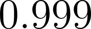 , so after 10,000 episodes it has decayed from
 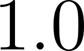 toward the floor of
 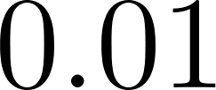 .
.
The Main Function
main wires everything together, prints the environment summary, trains the Q-table, then displays the learned greedy policy and a final held-out evaluation over 1000 episodes:
 1 (def (main)
 2   (let ((env (make-frozen-lake #t)))
 3     (displayln "=== Q-Learning on FrozenLake ===")
 4     (displayln (format "States: ~a, Actions: ~a" (hash-ref env 'n-states) (hash-ref env 'n-actions)))
 5     (displayln "")
 6     (displayln "Training:")
 7     (let* ((Q (q-learning env))
 8            (arrows '#("↑" "→" "↓" "←")))
 9       (displayln "")
10       (displayln "Learned policy:")
11       (do ((r 0 (+ r 1)))
12           ((= r 4))
13         (let ((line "  "))
14           (do ((c 0 (+ c 1)))
15               ((= c 4))
16             (let* ((s (+ (* r 4) c))
17                    (best-a (argmax (vector-ref Q s)))
18                    (arrow (vector-ref arrows best-a)))
19               (set! line (string-append line arrow))))
20           (displayln line)))
21
22       (displayln "")
23       (displayln (format "Final success rate (1000 episodes): ~a"
24                          (format-decimal (evaluate env Q 1000) 2))))))
25
26 (main)
Running the Q-Learning Demo
Because Q-learning involves random exploration and a stochastic environment, the exact numbers change on every run. A representative session looks like this:
 1 $ make run-qlearning
 2 gxi frozen_lake_qlearning.ss
 3 === Q-Learning on FrozenLake ===
 4 States: 16, Actions: 4
 5
 6 Training:
 7   Episode  1000: success = 0.72
 8   Episode  2000: success = 0.61
 9   Episode  3000: success = 0.77
10   Episode  4000: success = 0.74
11   Episode  5000: success = 0.73
12   Episode  6000: success = 0.44
13   Episode  7000: success = 0.70
14   Episode  8000: success = 0.76
15   Episode  9000: success = 0.71
16   Episode 10000: success = 0.71
17
18 Learned policy:
19   ←↑↑↑
20   ←↑←↑
21   ↑↓←↑
22   ↑→↓↑
23
24 Final success rate (1000 episodes): 0.79
Interpreting the Q-Learning Results
The most immediately surprising thing about the learned policy is that it does not look at all like “walk toward the goal”. Many cells appear to point away from the goal. This is the fingerprint of a policy that has learned to exploit the slipperiness of the ice.
Consider cell 0 (top-left), where the policy says LEFT. The agent obviously cannot walk further left than the wall. What actually happens is that pressing LEFT with slip probability yields:
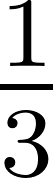 chance to actually go LEFT (stay in cell 0).
- chance to slip UP (also stay in cell 0).
- chance to slip DOWN (move to cell 4, a safe frozen cell).
The nominal “LEFT” action is really “make progress downward without ever risking a slip into the deadly hole at cell 5”. The agent has learned to use the wall to filter out dangerous slips. This is a classic and beautiful phenomenon in stochastic RL: the optimal action often has to be chosen for its distribution of outcomes rather than its intended direction.
Other observations:
- Success rates oscillate during training. Because is still positive, exploration occasionally overwrites good Q-values with noisy ones. This is unavoidable in tabular Q-learning without more advanced tricks like target networks or Double Q-learning.
- Final success rate around 0.75–0.80 is typical for this environment and this algorithm. The theoretical maximum success rate on slippery FrozenLake with a Q-learning agent is a bit above 0.80. Getting significantly higher requires either less slipperiness or more sophisticated algorithms.
- The learned policy is not unique. Repeated runs produce different arrangements of arrows, all of which are approximately optimal. Any two policies that agree on the “moves that trigger the right slip distribution” have roughly equal expected return.
Wrap Up
Value Iteration and Q-Learning are the two founding algorithms of reinforcement learning, and both fit comfortably into a few hundred lines of readable Gerbil Scheme. The exercise reveals several ideas that generalize far beyond these toy examples:
- Bellman equations turn planning into a fixed-point computation. Whenever you can write a recursive characterization of the value function, you can build a solver by iterating it.
- Model-free learning is simply model-based planning with a moving estimate. The Q-learning update rule is the Bellman update rule with the transition and reward model replaced by one sample of experience.
- Exploration is not a nuisance to be minimized, it is a first-class part of the algorithm.-greedy decay is a specific choice; entire subfields of RL exist to design better exploration strategies.
- Stochastic dynamics reward counterintuitive policies. Learning “walk away from the goal” is often correct on FrozenLake, because it neutralizes the slipperiness.
Gerbil Scheme’s combination of vectors, hash tables, and named let loops makes it a natural language for these numerical experiments. The imperative flavor of the code, with set! and vector-set!, may feel unusual to Schemers coming from a purely functional background, but it maps directly onto how these algorithms are described in textbooks and helps keep the code close to the theory.
Optional Practice Problems
Deterministic FrozenLake: Call
(make-frozen-lake #f)instead of(make-frozen-lake #t)and rerunq-learning. Report the final success rate and describe how the learned policy differs from the slippery case. Explain why the arrows now point unambiguously toward the goal.Sweep the Discount Factor: In
mdp_demo.ss, runvalue-iterationwithgammaset to0.5,0.7,0.9, and0.99. Report the number of iterations to convergence and the value at cell 0 for each. Explain the relationship between and convergence rate.Slower Epsilon Decay: Change the
decayargument inq-learningfrom0.999to0.9995and rerun. Does the final success rate improve? Does the training take noticeably longer to reach a stable policy? Explain how the exploration schedule affects sample efficiency.Add a Reward Shaper: Modify
frozen-lake-step!so that stepping onto a hole yields reward-1.0instead of0.0. Re-train and report how the learned policy changes. Discuss the tradeoffs of reward shaping versus letting the agent learn purely from the terminal +1 signal.Larger Grid World: Generalize
mdp_demo.ssfrom to 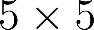 . Place a goal at the bottom-right corner, a trap somewhere in the interior, and run value iteration. Print the value function as a heat map (using formatted numbers in a grid layout) and the policy arrows side by side.
Q-Learning on the 3×3 Grid: Port the deterministic 3×3 grid world from
mdp_demo.ssinto a Q-learning environment analogous to FrozenLake and train a Q-table on it. Compare the learned policy and value estimates against the exact solution from Value Iteration. This exercise directly demonstrates the connection between model-free learning and model-based planning.Double Q-Learning: Q-learning is known to suffer from maximization bias: the
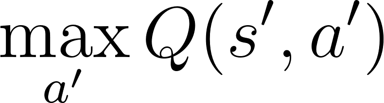 term systematically overestimates true action values. Implement Double Q-Learning, which maintains two independent Q-tables
 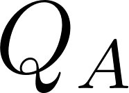 and
and 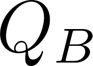 and uses one to select the greedy action and the other to evaluate it. Compare final success rates against vanilla Q-learning across ten training runs.
SARSA: Implement SARSA, the on-policy sibling of Q-learning. Instead of updating toward
, SARSA updates toward 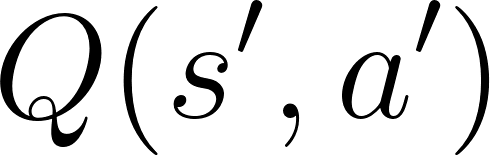 where
where 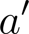 is the action actually taken by the current -greedy policy. Compare SARSA’s learned policy with Q-learning’s on slippery FrozenLake and explain any qualitative differences (SARSA is typically more conservative near cliffs and holes).