Gaussian Anomaly Detection
Anomaly detection is one of the most practical applications of unsupervised and semi-supervised machine learning. Please note dear reader that the next chapter introduces K-means that is another useful semi-supervised machine learning.
Rather than asking “what class does this belong to?”, we ask a subtler and often more useful question: “does this observation look like the ones I have already seen?” In fraud detection, manufacturing quality control, medical diagnostics, network intrusion monitoring, and predictive maintenance, the interesting events are usually rare. Trying to build a supervised classifier for events that occur one time in a thousand often fails: there are simply not enough positive examples to learn a good decision boundary. Anomaly detection sidesteps this problem entirely by modeling the normal distribution of data and flagging observations that fall outside it.
In this chapter we implement a multivariate Gaussian anomaly detector in Gerbil Scheme from scratch, then apply it to the classic Wisconsin Breast Cancer dataset. The detector fits a Gaussian distribution to each feature independently (a “diagonal covariance” assumption), computes the probability density 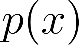 of each observation, and flags observations whose density falls below a threshold
  as anomalies. The threshold is selected automatically by sweeping over 200 candidate values and picking the one that maximizes performance on a cross-validation set.
Theoretical Background
The core idea is that if we assume each feature 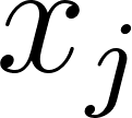 of a “normal” observation is drawn from a Gaussian distribution with mean
  and variance
 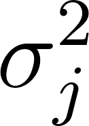 , then the probability density of a full observation vector
  can be approximated by combining the per-feature Gaussians. The Gaussian probability density function for a single feature is:

A standard multivariate Gaussian anomaly detector multiplies these per-feature densities together (assuming feature independence). The implementation in this chapter uses a slight variation: it computes the arithmetic mean of the per-feature PDFs rather than their product. This has the practical benefit of keeping the resulting numbers on a comfortable scale (avoiding vanishingly small products when there are many features) while still giving a monotone score suitable for thresholding.
The training procedure is straightforward:
- Split the examples into training (60%), cross-validation (20%), and test (~20%) sets. The training set is filtered to contain mostly normal examples.
- Fit the per-feature mean and variance using only the training set.
- Sweep many candidate values of and pick the one that yields the fewest misclassifications on the cross-validation set.
- Evaluate the final model on the held-out test set, reporting precision, recall, and
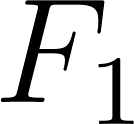 -score.
A key trick used here (following Andrew Ng’s classic Coursera Machine Learning lectures) is that we deliberately let a small number of anomalous examples leak into the CV and test sets - they are essential for tuning and for measuring recall.
The Dataset
We use the Wisconsin Breast Cancer Dataset, a well-known benchmark in medical machine learning. Each row is derived from a fine needle aspirate (FNA) of a breast mass and contains 9 cytological features scored on an integer scale from 1 to 10, plus a target label:
- Features (columns 1-9): clump thickness, uniformity of cell size, uniformity of cell shape, marginal adhesion, single epithelial cell size, bare nuclei, bland chromatin, normal nucleoli, mitoses.
- Target (column 10):
2for benign,4for malignant.
The raw CSV format is refreshingly simple. Here are the first few lines of data/cleaned_wisconsin_cancer_data.csv:
1 10,10,10,8,6,1,8,9,1,4
2 6,2,1,1,1,1,7,1,1,2
3 5,4,4,9,2,10,5,6,1,4
4 2,5,3,3,6,7,7,5,1,4
5 10,4,3,1,3,3,6,5,2,4
6 6,10,10,2,8,10,7,3,3,4
7 5,6,5,6,10,1,3,1,1,4
8 10,10,10,4,8,1,8,10,1,4
9 1,1,1,1,2,1,2,1,2,2
The final column of 2 or 4 is what we want to remap to {0.0, 1.0} so the detector can distinguish anomalies (malignant) from normals (benign).
Project Structure
The project directory source_code/anomaly-detection contains:
| File | Description |
|---|---|
detector.ss |
The anomaly detection engine: parameter fitting, PDF evaluation, threshold sweep, and model testing. |
wisconsin_demo.ss |
CSV loading, preprocessing, training, and end-to-end evaluation on the Wisconsin dataset. |
data/cleaned_wisconsin_cancer_data.csv |
The Wisconsin breast cancer dataset (648 examples). |
Makefile |
Single test target that invokes gxi wisconsin_demo.ss. |
gerbil.pkg |
Package declaration (anomaly-detection). |
The Detector Module: detector.ss
This module contains the entire anomaly detection engine. It has no dependency on the Wisconsin dataset - it can be reused for any labelled dataset in which the final column encodes the anomaly label as 1.0 (anomaly) or 0.0 (normal).
We start with the imports and exports. The :std/format module gives us format for printing, :std/pregexp is available for regex use in downstream modules, and :gerbil/gambit exposes the underlying Gambit runtime primitives.
 1 ;; File: detector.ss
 2 (import :std/format
 3         :std/pregexp
 4         :gerbil/gambit)
 5
 6 (export split-data
 7         compute-mu
 8         compute-sigma-sq
 9         gaussian-p
10         build-detector
11         train
12         is-anomaly
13         test-model
14         format-decimal)
15
16 (def SQRT_2_PI (sqrt (* 2.0 (acos -1.0))))
The constant SQRT_2_PI is precomputed once as 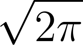 because it appears in the denominator of every Gaussian PDF evaluation. Note the small trick
 (acos -1.0) to obtain  without hardcoding a magic number.
Decimal Formatting Helpers
Gerbil’s default number printing yields long decimal expansions (like 0.8571428571428571), which are inconvenient for reporting metrics. The next two helpers give us format-decimal for pretty-printing floats to a fixed number of places:
 1 ;; Find index of character in string (helper for format-decimal)
 2 (def (string-index str char)
 3   (let ((len (string-length str)))
 4     (let loop ((i 0))
 5       (cond
 6         ((= i len) #f)
 7         ((char=? (string-ref str i) char) i)
 8         (else (loop (+ i 1)))))))
 9
10 ;; Format floating point numbers to a fixed number of decimal places
11 (def (format-decimal x places)
12   (let* ((multiplier (expt 10 places))
13          (rounded (/ (round (* x multiplier)) multiplier))
14          (str (number->string rounded)))
15     (let ((dot-pos (string-index str #\.)))
16       (let ((formatted-str
17              (if dot-pos
18                (let* ((frac-len (- (string-length str) dot-pos 1))
19                       (diff (- places frac-len)))
20                  (if (> diff 0)
21                    (string-append str (make-string diff #\0))
22                    str))
23                (string-append str "." (make-string places #\0)))))
24         (if (char=? (string-ref formatted-str 0) #\.)
25           (string-append "0" formatted-str)
26           formatted-str)))))
format-decimal multiplies by  , rounds to the nearest integer, divides back, then post-processes the string to zero-pad the fractional part and prepend a leading
 0 when necessary. The result is a stable, readable representation like "0.8571".
Splitting the Data
The split-data procedure randomly divides the examples into three sets. Crucially, it applies an additional filter to the training set: it accepts an example into training only if it is a normal one (target < 0.5), or with a small 10% probability if it is an anomaly. This mirrors the standard anomaly detection recipe - train primarily on normals, but keep some anomalies in CV and test for threshold tuning and evaluation.
 1 ;; Split examples into training (~60%), cross-validation (~20%), and test sets (~20%)
 2 (def (split-data examples num-features)
 3   (let ((train '())
 4         (cv '())
 5         (test '())
 6         (oi (- num-features 1)))
 7     (for-each
 8       (lambda (ex)
 9         (if (< (random-real) 0.6)
10           (when (or (< (vector-ref ex oi) 0.5) (< (random-real) 0.1))
11             (set! train (cons ex train)))
12           (if (< (random-real) 0.7)
13             (set! cv (cons ex cv))
14             (set! test (cons ex test)))))
15       examples)
16     `((train . ,(reverse train))
17       (cv . ,(reverse cv))
18       (test . ,(reverse test)))))
The function returns an association list keyed by 'train, 'cv, and 'test. Each example is a vector where index (- num-features 1) holds the target label.
Fitting Mean and Variance
Fitting is textbook: compute the sample mean and sample variance for each feature. compute-mu loops over all examples, accumulating a per-feature sum into a vector, then divides by the number of examples:
 1 ;; Per-feature mean mu
 2 (def (compute-mu examples nf)
 3   (let* ((mu (make-vector nf 0.0))
 4          (len (length examples)))
 5     (if (= len 0)
 6       mu
 7       (begin
 8         (for-each
 9           (lambda (ex)
10             (do ((f 0 (+ f 1)))
11                 ((= f nf))
12               (vector-set! mu f (+ (vector-ref mu f) (vector-ref ex f)))))
13           examples)
14         (do ((f 0 (+ f 1)))
15             ((= f nf) mu)
16           (vector-set! mu f (/ (vector-ref mu f) len)))))))
compute-sigma-sq follows the same shape but accumulates squared deviations from the mean. Note the small floor of 1.0e-10 to prevent divide-by-zero when a feature happens to be perfectly constant on the training set:
 1 ;; Per-feature variance sigmaSq
 2 (def (compute-sigma-sq examples mu nf)
 3   (let* ((s2 (make-vector nf 0.0))
 4          (len (length examples)))
 5     (do ((f 0 (+ f 1)))
 6         ((= f (- nf 1)) s2)
 7       (let ((sum-val 0.0))
 8         (for-each
 9           (lambda (ex)
10             (let* ((d (- (vector-ref ex f) (vector-ref mu f))))
11               (set! sum-val (+ sum-val (* d d)))))
12           examples)
13         (vector-set! s2 f (max (/ sum-val len) 1.0e-10))))))
Notice that the outer loop terminates at (- nf 1) rather than nf. This deliberately skips the last column (the target label) - we don’t want to include the label in the Gaussian model.
The Gaussian Score
The gaussian-p function computes the density score used for classification. As mentioned above, it takes the arithmetic mean of the per-feature Gaussian PDFs rather than their product. This is the score we will threshold with :
1 ;; Average Gaussian PDF p(x) across all features
2 (def (gaussian-p x mu sigma-sq nf)
3   (let ((sum-val 0.0))
4     (do ((f 0 (+ f 1)))
5         ((= f (- nf 1)) (/ sum-val nf))
6       (let* ((s2 (vector-ref sigma-sq f))
7              (d (- (vector-ref x f) (vector-ref mu f)))
8              (pdf (* (/ 1.0 (* SQRT_2_PI (sqrt s2))) (exp (- (/ (* d d) (* 2.0 s2)))))))
9         (set! sum-val (+ sum-val pdf))))))
Assembling the Detector
build-detector is the constructor. It takes raw labelled examples, splits them, computes  , and stashes everything into a hash table that carries the model state:
 1 ;; Build a detector from labelled examples
 2 (def (build-detector examples num-features)
 3   (let* ((split (split-data examples num-features))
 4          (train (cdr (assoc 'train split)))
 5          (cv (cdr (assoc 'cv split)))
 6          (test (cdr (assoc 'test split)))
 7          (mu (compute-mu train num-features))
 8          (sigma-sq (make-vector num-features 0.0))
 9          (ht (make-hash-table)))
10     (hash-put! ht 'num-features num-features)
11     (hash-put! ht 'mu mu)
12     (hash-put! ht 'sigma-sq sigma-sq)
13     (hash-put! ht 'best-eps 0.02)
14     (hash-put! ht 'training train)
15     (hash-put! ht 'cross-validation cv)
16     (hash-put! ht 'testing test)
17     ht))
The Threshold Sweep
The core of training is to try many candidate values of and pick the one that produces the fewest classification errors on the cross-validation set. train-helper recomputes 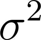 (from the training set) and counts CV errors for a given epsilon:
 1 (def (train-helper det epsilon)
 2   (let* ((nf (hash-ref det 'num-features))
 3          (training (hash-ref det 'training))
 4          (mu (hash-ref det 'mu))
 5          (cv (hash-ref det 'cross-validation))
 6          (sigma-sq (compute-sigma-sq training mu nf))
 7          (errors 0))
 8     (hash-put! det 'sigma-sq sigma-sq)
 9     (for-each
10       (lambda (x)
11         (let* ((prob (gaussian-p x mu sigma-sq nf))
12                (anomaly (> (vector-ref x (- nf 1)) 0.5)))
13           (if (if anomaly (> prob epsilon) (< prob epsilon))
14             (set! errors (+ errors 1))
15             #f)))
16       cv)
17     errors))
The subtle bit is the inner if: for a true anomaly, an error occurs when the score is above (we called it normal); for a true normal, an error occurs when the score is below (we called it anomalous).
Test-Set Evaluation
test-model runs the full confusion matrix on the held-out test set and prints precision, recall, and :
 1 ;; Evaluate model on test data
 2 (def (test-model det epsilon)
 3   (let* ((nf (hash-ref det 'num-features))
 4          (mu (hash-ref det 'mu))
 5          (sigma-sq (hash-ref det 'sigma-sq))
 6          (testing (hash-ref det 'testing))
 7          (tp 0) (fp 0) (fn 0) (tn 0))
 8     (for-each
 9       (lambda (x)
10         (let* ((prob (gaussian-p x mu sigma-sq nf))
11                (anomaly (> (vector-ref x (- nf 1)) 0.5)))
12           (if anomaly
13             (if (> prob epsilon) (set! fn (+ fn 1)) (set! tp (+ tp 1)))
14             (if (< prob epsilon) (set! fp (+ fp 1)) (set! tn (+ tn 1))))))
15       testing)
16     (let* ((precision (if (= (+ tp fp) 0) 0.0 (/ (exact->inexact tp) (+ tp fp))))
17            (recall (if (= (+ tp fn) 0) 0.0 (/ (exact->inexact tp) (+ tp fn))))
18            (f1 (if (= (+ precision recall) 0.0) 0.0 (/ (* 2.0 precision recall) (+ precision recall)))))
19       (displayln (format "\n -- best epsilon = ~a" (format-decimal epsilon 4)))
20       (displayln (format " -- test examples  = ~a" (length testing)))
21       (displayln (format " -- TP=~a FP=~a FN=~a TN=~a" tp fp fn tn))
22       (displayln (format " -- precision=~a recall=~a F1=~a"
23                          (format-decimal precision 4)
24                          (format-decimal recall 4)
25                          (format-decimal f1 4)))
26       `((precision . ,precision)
27         (recall . ,recall)
28         (f1 . ,f1)))))
The Top-Level Training Loop and Anomaly Predicate
Finally, train sweeps 200 values of starting from 0.001 in increments of 0.005, keeps the value that minimized CV errors, then evaluates on the test set:
 1 ;; Sweep 200 epsilon values, pick best, evaluate on test set
 2 (def (train det)
 3   (let ((best-err 1.0e10)
 4         (best-e 0.001))
 5     (do ((i 0 (+ i 1)))
 6         ((= i 200))
 7       (let* ((eps (+ 0.001 (* 0.005 i)))
 8              (err (train-helper det eps)))
 9         (when (<= err best-err)
10           (set! best-err err)
11           (set! best-e eps))))
12     (displayln (format "\n**** Best epsilon = ~a" (format-decimal best-e 4)))
13     (hash-put! det 'best-eps best-e)
14     (train-helper det best-e)
15     (test-model det best-e)
16     det))
17
18 ;; Return true if x is classified as an anomaly
19 (def (is-anomaly det x)
20   (< (gaussian-p x (hash-ref det 'mu) (hash-ref det 'sigma-sq) (hash-ref det 'num-features))
21      (hash-ref det 'best-eps)))
is-anomaly is the user-facing predicate: given a trained detector and a new observation vector, return #t if the Gaussian score falls below the learned threshold.
The Demo Program: wisconsin_demo.ss
The demo file glues the detector to the Wisconsin dataset. It imports the detector module (via the sibling filename import "detector") plus a few standard modules for I/O and regex splitting:
1 ;; File: wisconsin_demo.ss
2 (import "detector")
3 (import :std/misc/ports
4         :std/pregexp
5         :std/format
6         :gerbil/gambit)
Loading CSV Data
load-csv reads the file line-by-line, trims whitespace, splits on commas, converts each token to a number, and returns a list of vectors:
 1 ;; Trim leading and trailing whitespace
 2 (def (string-trim str)
 3   (pregexp-replace "^\\s+" (pregexp-replace "\\s+$" str "") ""))
 4
 5 (def (load-csv path)
 6   (let ((lines (read-file-lines path)))
 7     (let loop ((lines lines) (acc '()))
 8       (if (null? lines)
 9         (reverse acc)
10         (let* ((line (string-trim (car lines)))
11                (trimmed-len (string-length line)))
12           (if (> trimmed-len 0)
13             (let* ((tokens (pregexp-split "," line))
14                    (numbers (map string->number tokens))
15                    (vec (list->vector numbers)))
16               (loop (cdr lines) (cons vec acc)))
17             (loop (cdr lines) acc)))))))
Empty lines are silently skipped, which makes the loader forgiving of trailing newlines.
Preprocessing the Wisconsin Rows
Raw integer scores from 1 to 10 are not ideal for Gaussian modeling - the features are heavily skewed, with many observations pinned at 1. The preprocessing pipeline in preprocess-wisconsin applies three transformations to each row:
- Scale down the raw features (indices 0-8) by 0.1, moving them into a smaller numeric range.
- Log-transform each feature as
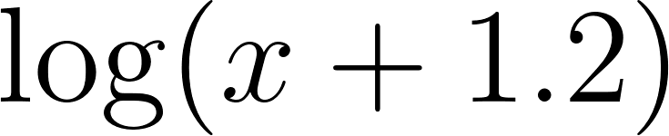 . The additive constant prevents
  and softens the tail.
- Per-row min-max scale the features to the interval
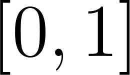 , so no feature dominates the Gaussian by virtue of its raw magnitude.
The target column is separately remapped from 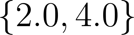 to
to 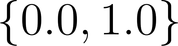 :
:
 1 ;; Log-transform, per-row min-max scaling, remap target {2,4} -> {0,1}
 2 (def (preprocess-wisconsin rows)
 3   (map
 4     (lambda (row)
 5       (let* ((xs (make-vector 10 0.0))
 6              (mn 1.0e9)
 7              (mx -1.0e9))
 8         ;; Multiply feature values (indices 0 to 8) by 0.1
 9         (do ((i 0 (+ i 1)))
10             ((= i 9))
11           (vector-set! xs i (* (vector-ref row i) 0.1)))
12         ;; Copy target (index 9)
13         (vector-set! xs 9 (vector-ref row 9))
14
15         ;; Compute log and find min/max
16         (do ((i 0 (+ i 1)))
17             ((= i 9))
18           (let ((v (log (+ (vector-ref xs i) 1.2))))
19             (vector-set! xs i v)
20             (when (< v mn) (set! mn v))
21             (when (> v mx) (set! mx v))))
22
23         ;; Min-max scale the features
24         (let ((range (- mx mn)))
25           (do ((i 0 (+ i 1)))
26               ((= i 9))
27             (if (< range 1.0e-10)
28               (vector-set! xs i 0.5)
29               (vector-set! xs i (/ (- (vector-ref xs i) mn) range)))))
30
31         ;; Normalize target from {2.0, 4.0} to {0.0, 1.0}
32         (vector-set! xs 9 (* (- (vector-ref xs 9) 2.0) 0.5))
33         xs))
34     rows))
The Main Entry Point
The main function ties everything together: load the CSV, preprocess, build the detector, train it (which internally sweeps and evaluates on test), then run a couple of light sanity checks:
 1 (def (main)
 2   (let* ((data (preprocess-wisconsin (load-csv "data/cleaned_wisconsin_cancer_data.csv"))))
 3     (displayln (format "Loaded ~a examples." (length data)))
 4
 5     (let* ((det (build-detector data 10)))
 6       (displayln (format "\nTraining set:  ~a" (length (hash-ref det 'training))))
 7       (displayln (format "Cross-val set: ~a" (length (hash-ref det 'cross-validation))))
 8       (displayln (format "Test set:      ~a" (length (hash-ref det 'testing))))
 9
10       (train det)
11
12       (displayln (format "\nModel: bestEps=~a, features=~a"
13                          (format-decimal (hash-ref det 'best-eps) 4)
14                          (hash-ref det 'num-features)))
15
16       ;; Assertions
17       (unless (> (hash-ref det 'best-eps) 0.0)
18         (error "epsilon should be positive"))
19       (unless (= (vector-length (hash-ref det 'mu)) 10)
20         (error "mu should have 10 elements"))
21
22       (let ((testing (hash-ref det 'testing)))
23         (when (> (length testing) 0)
24           (let* ((s (car testing))
25                  (actual (if (> (vector-ref s 9) 0.5) "anomaly" "normal"))
26                  (predicted (if (is-anomaly det s) "anomaly" "normal")))
27             (displayln (format "\nFirst test sample: actual=~a, predicted=~a" actual predicted)))))
28
29       (displayln "All assertions passed.")
30       (displayln "=== Test complete ==="))))
31
32 (main)
Running the Demo
Run either make test or invoke the interpreter directly. The Makefile is minimal:
1 test:
2     gxi wisconsin_demo.ss
A typical run produces output similar to the following. Because split-data uses random sampling, the exact numbers will vary from run to run:
 1 $ make test
 2 gxi wisconsin_demo.ss
 3 Loaded 648 examples.
 4
 5 Training set:  259
 6 Cross-val set: 188
 7 Test set:      68
 8
 9 **** Best epsilon = 0.8910
10
11  -- best epsilon = 0.8910
12  -- test examples  = 68
13  -- TP=24 FP=4 FN=1 TN=39
14  -- precision=0.8571 recall=0.9600 F1=0.9057
15
16 Model: bestEps=0.8910, features=10
17
18 First test sample: actual=anomaly, predicted=anomaly
19 All assertions passed.
20 === Test complete ===
Interpreting the Results
The output reports several important quantities.
- Loaded 648 examples: the total number of records read from the CSV.
- Training / Cross-val / Test set sizes: notice that the training set is smaller than a naive 60% split would give. That is expected -
split-datadeliberately drops most of the anomalous rows from the training set so the model learns what “normal” looks like. - Best epsilon = 0.8910: the classification threshold selected by the sweep. Any observation whose Gaussian score falls below
0.8910is flagged as an anomaly. - TP=24 FP=4 FN=1 TN=39: the confusion matrix on the 68-observation test set.
TP(true positive) is a correctly-identified malignant case,FN(false negative) is a missed malignant case,FP(false positive) is a benign case wrongly flagged, andTN(true negative) is a correctly-identified benign case. - precision = 0.8571: of the 28 observations the model called “anomaly”, 24 were truly malignant. Precision answers “when the model raises an alarm, how often is it right?”
- recall = 0.9600: of the 25 truly malignant observations, the model caught 24. Recall answers “of all the actual anomalies, how many did we catch?”
- F_1 = 0.9057: the harmonic mean of precision and recall.
F_1is a single-number summary of overall detection quality when both false positives and false negatives matter.
The recall value is particularly encouraging in a medical setting - missing a malignant tumor is a much more costly mistake than a false alarm, so a recall above 0.95 is a genuinely useful outcome.
Wrap Up
We built a full-featured Gaussian anomaly detection engine in Gerbil Scheme in fewer than 200 lines of code. The key ideas transfer to any application where “the interesting event is rare”:
- Fit a Gaussian per feature on your normal data.
- Use the density function as a score.
- Use a held-out cross-validation set with a few real anomalies in it to pick the best classification threshold.
- Report precision, recall, and on a completely held-out test set.
Gerbil Scheme turns out to be a comfortable environment for this kind of numerical work. Vectors give us cheap random-access storage, hash tables give us a natural home for the trained model’s state, and the top-level def / import / export module system keeps detector.ss cleanly reusable across different datasets. Try pointing wisconsin_demo.ss at your own CSV data - as long as the last column is a binary anomaly label, the detector will happily consume it.
Optional Practice Problems
Product-of-PDFs Score:
gaussian-pcurrently returns the arithmetic mean of the per-feature PDFs. Add a new functiongaussian-p-productthat instead returns the classical multivariate Gaussian score (the product of the per-feature PDFs) and compare its precision/recall/F1 against the mean-based score on the Wisconsin dataset.Sensitivity to the Preprocessing Pipeline: In
preprocess-wisconsin, remove the log-transform step (leave only the*0.1scaling and the min-max normalization). Re-run the demo and report how the best, precision, recall, and change. Explain why the log-transform helps or hurts.Configurable Sweep Range: Modify
trainindetector.ssto accept optional keyword argumentseps-start,eps-step, andeps-countso users can control the epsilon sweep without editing the source. Provide sensible defaults matching the current behavior (0.001, 0.005, 200).Save and Load a Trained Detector: Implement
save-detectorandload-detectorfunctions indetector.ssthat serialize the trained, , best-eps, andnum-featuresto a plain-text file and read them back in a later session, so that training does not need to be repeated to classify new observations.Try a Different Dataset: The KDD Cup 1999 network intrusion dataset is a classic benchmark for anomaly detection. Write a
kdd_demo.ssthat mimicswisconsin_demo.ssfor a subset of the KDD data, including any needed preprocessing (categorical features must be converted to numeric form). Report how well the detector performs.