3. Compiling Python Source Code

Although most people may not regard Python as a compiled language, it is one. During compilation, the interpreter generates executable bytecode from Python source code. However, Python’s compilation process is a relatively simple one. It involves the following steps in order.

1. Parsing the source code into a parse tree.
2. Transforming the parse tree into an abstract syntax tree (AST).
3. Generating the symbol table.
4. Generating the code object from the AST. This step involves:
   1. Transforming the AST into a flow control graph, and
   2. Emitting a code object from the control flow graph.

Parsing source code into a parse tree and creating an AST from such a parse is a standard process and Python does not introduce any complicated nuances, so the focus of this chapter is on the transformation of an AST into a control flow graph and the emission of code object from the control flow graph. For anyone interested in parse tree and AST generation, the dragon book provides an in-depth tour de force of both topics.

3.1 From Source To Parse Tree

The Python parser is an LL(1) parser based on the description of such parsers laid out in the Dragon book. The Grammar/Grammar module contains the Extended Backus-Naur Form (EBNF) grammar specification of the Python language. Listing 3.0 is a cross-section of this grammar.

 1 stmt: simple_stmt | compound_stmt
 2 simple_stmt: small_stmt (';' small_stmt)* [';'] NEWLINE
 3 small_stmt: (expr_stmt | del_stmt | pass_stmt | flow_stmt |
 4         import_stmt | global_stmt | nonlocal_stmt | assert_stmt)
 5 expr_stmt: testlist_star_expr (augassign (yield_expr|testlist) |
 6                 ('=' (yield_expr|testlist_star_expr))*)
 7 testlist_star_expr: (test|star_expr) (',' (test|star_expr))* [',']
 8 augassign: ('+=' | '-=' | '*=' | '@=' | '/=' | '%=' | '&=' | '|=' | '^=' 
 9         | '<<=' | '>>=' | '**=' | '//=')
10 
11 del_stmt: 'del' exprlist
12 pass_stmt: 'pass'
13 flow_stmt: break_stmt | continue_stmt | return_stmt | raise_stmt | 
14         yield_stmt
15 break_stmt: 'break'
16 continue_stmt: 'continue'
17 return_stmt: 'return' [testlist]
18 yield_stmt: yield_expr
19 raise_stmt: 'raise' [test ['from' test]]
20 import_stmt: import_name | import_from
21 import_name: 'import' dotted_as_names
22 import_from: ('from' (('.' | '...')* dotted_name | ('.' | '...')+)
23         'import' ('*' | '(' import_as_names ')' | import_as_names))
24 import_as_name: NAME ['as' NAME]
25 dotted_as_name: dotted_name ['as' NAME]
26 import_as_names: import_as_name (',' import_as_name)* [',']
27 dotted_as_names: dotted_as_name (',' dotted_as_name)*
28 dotted_name: NAME ('.' NAME)*
29 global_stmt: 'global' NAME (',' NAME)*
30 nonlocal_stmt: 'nonlocal' NAME (',' NAME)*
31 assert_stmt: 'assert' test [',' test]
32 
33         ...

The PyParser_ParseFileObject function in Parser/parsetok.c is the entry point for parsing any module passed to the interpreter at the command-line. This function invokes the PyTokenizer_FromFile function that is responsible for generating tokens from the supplied modules.

3.2 Python tokens

Python source code consists of tokens. For example, return is a keyword token; 2 is a literal numeric token. Tokenization, the splitting of source code into constituent tokens, is the first task during parsing. The tokens from this step fall into the following categories.

1. identifiers: These are names defined by a programmer. They include function names, variable names, class names, etc. These must conform to the rules of identifiers specified in the Python documentation.
2. operators: These are special symbols such as +, * that operate on data values, and produce results.
3. delimiters: This group of symbols serve to group expressions, provide punctuations, and assignment. Examples in this category include (, ), {,}, =, *= etc.
4. literals: These are symbols that provide a constant value for some type. We have the string and byte literals such as "Fred", b"Fred" and numeric literals which include integer literals such as 2, floating-point literal such as 1e100 and imaginary literals such as 10j.
5. comments: These are string literals that start with the hash symbol. Comment tokens always end at the end of the physical line.
6. NEWLINE: This is a unique token that denotes the end of a logical line.
7. INDENT and DEDENT: These token represent indentation levels that group compound statements.

A group of tokens delineated by the NEWLINE token makes up a logical line; hence we could say that a Python program consists of a sequence of logical lines. Each of these logical lines consists of several physical lines that are each terminated by an end-of-line sequence. Most times, logical lines map to physical lines, so we have a logical line delimited by end-of-line characters. These logical lines usually map to Python statements. Compound statements may span multiple physical lines; parenthesis, square brackets or curly braces around a statement implicitly joins the logical lines that make up such statement. The backslash character, on the other hand, is needed to join multiple logical lines explicitly.

Indentation also plays a central role in grouping Python statements. One of the lines in the Python grammar is thus suite: simple_stmt | NEWLINE INDENT stmt+ DEDENT so a crucial task of the tokenizer generating indent and dedent tokens that go into the parse tree. The tokenizer uses an algorithm similar to that in Listing 3.1 to generate these INDENT and DEDENT tokens.

 1 Init the indent stack with the value 0.
 2 For each logical line taking into consideration line-joining:
 3     A.  If the current line's indentation is greater than the 
 4     indentation at the top of the stack
 5         1.  Add the current line's indentation to the top of the stack.
 6         2.  Generate an INDENT token.
 7     B.  If the current line's indentation is less than the indentation
 8         at the top of the stack
 9         1. If there is no indentation level on the stack that matches the current li\
10 ne's indentation, report an error.
11         2.  For each value at the top of the stack, that is unequal to the current l\
12 ine's indentation.
13             a.  Remove the value from the top of the stack.
14             b.  Generate a DEDENT token.
15     C.  Tokenize the current line.
16 For every indentation on the stack except 0, produce a DEDENT token.

The PyTokenizer_FromFile function in the Parser/tokenizer.c scans the source file from left to right and top to bottom tokenizing the file’s contents and then outputting a tokenizer structure. Whitespaces characters other than terminators serve to delimit tokens but are not compulsory. In cases of ambiguity such as in 2+2, a token comprises the longest possible string that forms a legal token reading from left to right; in this example, the tokens are the literal 2, the operator + and the literal 2.

The tokenizer structure generated by the PyTokenizer_FromFile function gets passed to the parsetok function that attempts to build a parse tree according to the Python grammar of which Listing 3.0 is a subset. When the parser encounters a token that violates the Python grammar, it raises a SyntaxError exception. The parser module provides limited access to the parse tree of a block of Python code, and listing 3.2 is a basic demonstration.

 1 >>>code_str = """def hello_world():
 2                     return 'hello world'
 3                 """
 4 >>> import parser
 5 >>> from pprint import pprint 
 6 >>> st = parser.suite(code_str)
 7 >>> pprint(parser.st2list(st))
 8 [257,
 9 [269,
10 [294,
11 [263,
12     [1, 'def'],
13     [1, 'hello_world'],
14     [264, [7, '('], [8, ')']],
15     [11, ':'],
16     [303,
17     [4, ''],
18     [5, ''],
19     [269,
20     [270,
21     [271,
22         [277,
23         [280,
24         [1, 'return'],
25         [330,
26         [304,
27             [308,
28             [309,
29             [310,
30             [311,
31                 [314,
32                 [315,
33                 [316,
34                 [317,
35                     [318,
36                     [319,
37                     [320,
38                     [321,
39                         [322, [323, [3, '"hello world"']]]]]]]]]]]]]]]]]]]],
40     [4, '']]],
41     [6, '']]]]],
42 [4, ''],
43 [0, '']]
44 >>>  

The parser.suite(source) call in listing 3.2 returns an intermediate representation of a parse tree (ST) object while the call to parser.st2list returns the parse tree represented by a Python list - each list represents a node of the parse tree. The first items in each list, the integer, identifies the production rule in the Python grammar responsible for that node.

Figure 3.0 is a tree diagram of the same parse tree from listing 3.2 with some tokens stripped away, and one can see more easily the part of the grammar each of the integer value represents. These production rules are all specified in the Include/token.h (terminals) and Include/graminit.h (terminals) header files.

3.3 From Parse Tree To Abstract Syntax Tree

The parse tree is dense with information about Python’s syntax, and all that information such as how lines are delimited is irrelevant for generating bytecode. This is where the abstract syntax tree (AST) comes in. The abstract syntax tree is a representation of the code that is independent of Python’s syntax niceties. For example, a parse tree contains syntax constructs such as colon and NEWLINE nodes, as shown in figure 3.0, but the AST does not include such syntax construct as shown in listing 3.4. The transformation of the parse tree to the abstract syntax tree is the next step in the compilation pipeline.

1 >>> import ast
2 >>> import pprint
3 >>> node = ast.parse(code_str, mode="exec")
4 >>> ast.dump(node)
5 ("Module(body=[FunctionDef(name='hello_world', args=arguments(args=[], "
6 'vararg=None, kwonlyargs=[], kw_defaults=[], kwarg=None, defaults=[]), '
7 "body=[Return(value=Str(s='hello world'))], decorator_list=[], "
8 'returns=None)])')

Python makes use of the Zephyr Abstract Syntax Definition Language (ASDL), and the ASDL definitions of the various Python constructs are in the file Parser/Python.asdl file. Listing 3.5 is a fragment of the ASDL definition of a Python statement.

 1 stmt = FunctionDef(identifier name, arguments args,
 2                    stmt* body, expr* decorator_list, expr? returns)
 3       | AsyncFunctionDef(identifier name, arguments args,
 4                          stmt* body, expr* decorator_list, expr? returns)
 5 
 6       | ClassDef(identifier name,
 7          expr* bases,
 8          keyword* keywords,
 9          stmt* body,
10          expr* decorator_list)
11       | Return(expr? value)
12 
13       | Delete(expr* targets)
14       | Assign(expr* targets, expr value)
15       | AugAssign(expr target, operator op, expr value)
16       -- 'simple' indicates that we annotate simple name without parens
17       | AnnAssign(expr target, expr annotation, expr? value, int simple)
18 
19       -- use 'orelse' because else is a keyword in target languages
20       | For(expr target, expr iter, stmt* body, stmt* orelse)
21       | AsyncFor(expr target, expr iter, stmt* body, stmt* orelse)
22       | While(expr test, stmt* body, stmt* orelse)
23       | If(expr test, stmt* body, stmt* orelse)
24       | With(withitem* items, stmt* body)
25       | AsyncWith(withitem* items, stmt* body)

The PyAST_FromNode function in the Python/ast.c calls PyAST_FromNodeObject also in Python/ast.c which walks the various parse tree nodes and generates AST nodes accordingly using functions defined in Python/ast.c. The heart of this function is a large switch statement that calls node specific functions on each node type. For example, the code responsible for generating the AST node for an if expression is in listing 3.7.

 1 static expr_ty
 2 ast_for_ifexpr(struct compiling *c, const node *n)
 3 {
 4     /* test: or_test 'if' or_test 'else' test */
 5     expr_ty expression, body, orelse;
 6 
 7     assert(NCH(n) == 5);
 8     body = ast_for_expr(c, CHILD(n, 0));
 9     if (!body)
10         return NULL;
11     expression = ast_for_expr(c, CHILD(n, 2));
12     if (!expression)
13         return NULL;
14     orelse = ast_for_expr(c, CHILD(n, 4));
15     if (!orelse)
16         return NULL;
17     return IfExp(expression, body, orelse, LINENO(n), n->n_col_offset,
18                  c->c_arena);
19 }

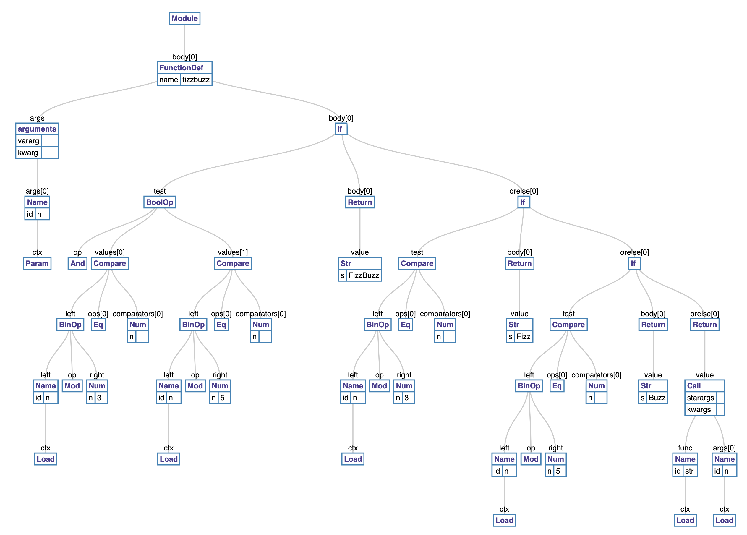
1 def fizzbuzz(n):
2     if n % 3 == 0 and n % 5 == 0:
3         return 'FizzBuzz'
4     elif n % 3 == 0:
5         return 'Fizz'
6     elif n % 5 == 0:
7         return 'Buzz'
8     else:
9         return str(n)

Take the code in Listing 3.8, for example, the transformation of its parse tree to an AST will result in an AST similar to figure 3.1.

The ast module bundled with the Python interpreter provides us with the ability to manipulate a Python AST. Tools such as codegen can take an AST representation in Python and output the corresponding Python source code.

With the AST generated, the next step is creating the symbol table.

3.4 Building The Symbol Table

The symbol table, as the name suggests, is a collection of symbols and their use context within a code block. Building the symbol table involves analyzing and assigning scoping to the names in a code block.

The PySymtable_BuildObject function in Python/compile.c walks the AST to create the symbol table. This is a two-step process summarized in listing 3.12.

For each node in a given AST
    If the node is the start of a code block:
        1. Create a new symbol table entry and set the current symbol table to this \
value. 
        2. Push the new symbol table to st_stack.
        3. Add the new symbol table to the list of children of the previous symbol t\
able.
        4. Update the current symbol table to this new symbol table
        5. For all nodes in the code block nodes: 
            a. recursively visit each node using the "symtable_visit_XXX" 
                functions where "XXX" is a node type.
        6. Exit the code block by removing the current symbol table entry from the s\
tack.
        7. Pop the next symbol table entry from the stack and set the 
        current symbol table entry to this popped value
    else:
        recursively visit the node and sub-nodes.

First, we visit each node of the AST to build a collection of symbols used. After the first pass, the symbol table entries contain all names that have been used within the module, but it does not have contextual information about such names. For example, the interpreter cannot tell if a given variable is a global, local, or free variable. The symtable_analyze function in the Parser/symtable.c handles the second phase. In this phase, the algorithm assigns scopes (local, global, or free) to the symbols gathered from the first pass. The comments in the Parser/symtable.c are quite informative and are paraphrased below to provide some insight into the second phase of the symbol table construction process.

The symbol table requires two passes to determine the scope of each name. The first pass collects raw facts from the AST via the symtable_visit_* functions while the second pass analyzes these facts during a pass over the PySTEntryObjects created during pass 1. During the second pass, the parent passes the set of all name bindings visible to its children when it enters a function. These bindings determine if nonlocal variables are free or implicit globals. Names which are explicitly declared nonlocal must exist in this set of visible names - if they do not, the interpreter raises a syntax error. After the local analysis, it analyzes each of its child blocks using an updated set of name bindings.

There are also two kinds of global variables, implicit and explicit. An explicit global is declared with the global statement. An implicit global is a free variable for which the compiler has found no binding in an enclosing function scope. The implicit global is either a global or a builtin.
Python’s module and class blocks use the xxx_NAME opcodes to handle these names to implement slightly odd semantics. In such a block, the name is treated as global until it is assigned a value; then it is treated like a local.

The children update the free variable set. If a child adds a variable to the set of free variables, then such variable is marked as a cell. The function object defined must provide runtime storage for the variable that may outlive the function’s frame. Cell variables are removed from the free set before the analyze function returns to its parent.

For example, a symbol table for a module with content in listing 3.16 will contain three symbol table entries.

def make_counter():
    count = 0
    def counter():
        nonlocal count 
        count += 1
        return count
    return counter

The first entry is that of the enclosing module, and it will have make_counter defined with a local scope. The next symbol table entry will be that of function make_counter, and this will have the count and counter names marked as local. The final symbol table entry will be that of the nested counter function. This entry will have the count variable marked as free. One thing to note is that although make_counter has a local scope in the symbol table entry for the module block, it is globally defined in the module code block because the *st_global field of the symbol table points to the *st_top symbol table entry which is that of the enclosing module.

3.5 From AST To Code Objects

After generating the symbol table, the next step is creating code objects. The functions for this step are in the Python/compile.c module. First, they convert the AST into basic blocks of Python byte code instructions. Basic blocks are blocks of code that have a single entry but can have multiple exits. The algorithm here uses a pattern similar to that used to generate the symbol table. Functions named compiler_visit_xx, where xx is the node type, recursively visit each node of the AST emitting bytecode instructions in the process. We see some examples of these functions in the sections that follow. The blocks of bytecode here implicitly represent a graph, the control flow graph. This graph shows the potential code execution paths. In the second step, the algorithm flattens the control flow graph using a post-order depth-first search transversal. After, the jump offsets are calculated and used as instruction arguments for bytecode jump instructions. The bytecode instructions are then used to create a code object.

Basic blocks

The basic block is central to generating code objects. A basic block is a sequence of instructions that has one entry point but multiple exit points. Listing 3.19 is the definition of the basic_block data structure.

 1 typedef struct basicblock_ {
 2     /* Each basicblock in a compilation unit is linked via b_list in the
 3     reverse order that the block are allocated.  b_list points to the next
 4     block, not to be confused with b_next, which is next by control flow. */
 5     struct basicblock_ *b_list;
 6     /* number of instructions used */
 7     int b_iused;
 8     /* length of instruction array (b_instr) */
 9     int b_ialloc;
10     /* pointer to an array of instructions, initially NULL */
11     struct instr *b_instr;
12     /* If b_next is non-NULL, it is a pointer to the next
13     block reached by normal control flow. */
14     struct basicblock_ *b_next;
15     /* b_seen is used to perform a DFS of basicblocks. */
16     unsigned b_seen : 1;
17     /* b_return is true if a RETURN_VALUE opcode is inserted. */
18     unsigned b_return : 1;
19     /* depth of stack upon entry of block, computed by stackdepth() */
20     int b_startdepth;
21     /* instruction offset for block, computed by assemble_jump_offsets() */
22     int b_offset;
23 } basicblock;

The interesting fields here are *b_list that is a linked list of all basic blocks allocated during the compilation process, *b_instr which is an array of instructions within the basic block and *b_next which is the next basic flow reached by normal control flow execution. Each instruction has a structure shown in Listing 3.20 that holds a bytecode instruction. These bytecode instructions are in the Include/opcode.h header file.

1 struct instr {
2     unsigned i_jabs : 1;
3     unsigned i_jrel : 1;
4     unsigned char i_opcode;
5     int i_oparg;
6     struct basicblock_ *i_target; /* target block (if jump instruction) */
7     int i_lineno;
8 };

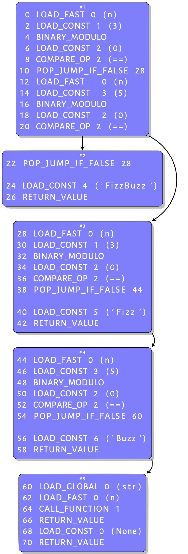
To illustrate how the interpreter creates these basic blocks, we use the function in Listing 3.11. Compiling its AST shown in figure 3.2 into a CFG results in the graph similar to that in figure 3.4 - this shows only blocks with instructions. An inspection of this graph provides some intuition behind the basic blocks. Some basic blocks have a single entry point, but others have multiple exits. These blocks are described in more detail next.

 1 static int
 2 compiler_if(struct compiler *c, stmt_ty s)
 3 {
 4     basicblock *end, *next;
 5     int constant;
 6     assert(s->kind == If_kind);
 7     end = compiler_new_block(c);
 8     if (end == NULL)
 9         return 0;
10 
11     constant = expr_constant(c, s->v.If.test);
12     /* constant = 0: "if 0"
13      * constant = 1: "if 1", "if 2", ...
14      * constant = -1: rest */
15     if (constant == 0) {
16         if (s->v.If.orelse)
17             VISIT_SEQ(c, stmt, s->v.If.orelse);
18     } else if (constant == 1) {
19         VISIT_SEQ(c, stmt, s->v.If.body);
20     } else {
21         if (asdl_seq_LEN(s->v.If.orelse)) {
22             next = compiler_new_block(c);
23             if (next == NULL)
24                 return 0;
25         }
26         else
27             next = end;
28         VISIT(c, expr, s->v.If.test);
29         ADDOP_JABS(c, POP_JUMP_IF_FALSE, next);
30         VISIT_SEQ(c, stmt, s->v.If.body);
31         if (asdl_seq_LEN(s->v.If.orelse)) {
32             ADDOP_JREL(c, JUMP_FORWARD, end);
33             compiler_use_next_block(c, next);
34             VISIT_SEQ(c, stmt, s->v.If.orelse);
35         }
36     }
37     compiler_use_next_block(c, end);
38     return 1;
39 }

The body of the function in Listing 3.13 is an if statement as is visible in figure 3.2. The snippet in Listing 3.21 is the function that compiles an if statement AST node into basic blocks. When this function compiles our example if statement node, the else statement on line 20 is executed. First, it creates a new basic block for an else node if such exists. Then, it visits the guard clause of the if statement node. What we have in the function in Listing 3.11 is interesting because the guard clause is a boolean expression which can trigger a jump during execution. Listing 3.22 is the function that compiles a boolean expression.

 1 static int compiler_boolop(struct compiler *c, expr_ty e)
 2 {
 3     basicblock *end;
 4     int jumpi;
 5     Py_ssize_t i, n;
 6     asdl_seq *s;
 7 
 8     assert(e->kind == BoolOp_kind);
 9     if (e->v.BoolOp.op == And)
10         jumpi = JUMP_IF_FALSE_OR_POP;
11     else
12         jumpi = JUMP_IF_TRUE_OR_POP;
13     end = compiler_new_block(c);
14     if (end == NULL)
15         return 0;
16     s = e->v.BoolOp.values;
17     n = asdl_seq_LEN(s) - 1;
18     assert(n >= 0);
19     for (i = 0; i < n; ++i) {
20         VISIT(c, expr, (expr_ty)asdl_seq_GET(s, i));
21         ADDOP_JABS(c, jumpi, end);
22     }
23     VISIT(c, expr, (expr_ty)asdl_seq_GET(s, n));
24     compiler_use_next_block(c, end);
25     return 1;
26 }

The code up to the loop at line 20 is straight forward. In the loop, the compiler visits each expression, and after each visit, it adds a jump. This is because of the short circuit evaluation used by Python. It means that when a boolean operation such as an AND evaluates to false, the interpreter ignores the other expressions and performs a jump to continue execution. The compiler knows where to jump to if need be because the following instructions go into a new basic block - the use of compiler_use_next_block enforces this. So we have two blocks now. After visiting the test, the compiler_if function adds a jump instruction for the if statement, then compiles the body of the if statement. Recall that after visiting the boolean expression, the compiler created a new basic block. This block contains the jump and instructions for body of the if statement, a simple return in this case. The target of this jump is the next block that will hold the elif arm of the if statement. The next step is to compile the elif component of the if statement but before this, the compiler calls the compiler_use_next_block function to activate the next block. The orElse arm is just another if statement, so the compiler_if function gets called again. This time around the test of the if is a compare operation. This is a single comparison, so there are no jumps involved and no new blocks, so the interpreter emits byte code for comparing values and returns to compile the body of the if statement. The same process continues for the last orElse arm resulting in the CFG in figure 3.3.

Figure 3.3 shows that the fizzbuzz function can exit block 1 in two ways. The first is via serial execution of all the instructions in block 1 then continuing in block 2. The other is via the jump instruction after the first compare operation. The target of this jump is block 3, but an executing code object knows nothing of basic blocks – the code object has a stream of bytecodes that are indexed with offsets. We have to provide the jump instructions with the offset into the bytecode instruction stream of the jump targets.

Assembling the basic blocks

The assemble function in Python/compile.c linearizes the CFG and creates the code object from the linearized CFG. It does so by computing the instruction offset for jump targets and using these as arguments to the jump instructions.

First, the assemble function, in this case, adds instructions for a return None statement since the last statement of the function is not a RETURN statement - now you know why you can define methods without adding a RETURN statement. Next, it flattens the CFG using a post-order depth-first traversal - the post-order traversal visits the children of a node before visiting the node itself. The assembler data structure holds the flattened graph, [block 5, block 4, block 3, block 2, block 1], in the a_postorder array for further processing. Next, it computes the instruction offsets and uses those as targets for the bytecode jump instructions. The assemble_jump_offsets function in listing 3.24 handles this.

The assemble_jump_offsets function in Listing 3.24 is relatively straightforward. In the for...loop at line 10, it computes the offset into the instruction stream for every instruction (akin to an array index). In the next for...loop at line 17, it uses the computed offsets as arguments to the jump instructions distinguishing between absolute and relative jumps.

 1 static void assemble_jump_offsets(struct assembler *a, struct compiler *c){
 2     basicblock *b;
 3     int bsize, totsize, extended_arg_recompile;
 4     int i;
 5 
 6     /* Compute the size of each block and fixup jump args.
 7        Replace block pointer with position in bytecode. */
 8     do {
 9         totsize = 0;
10         for (i = a->a_nblocks - 1; i >= 0; i--) {
11             b = a->a_postorder[i];
12             bsize = blocksize(b);
13             b->b_offset = totsize;
14             totsize += bsize;
15         }
16         extended_arg_recompile = 0;
17         for (b = c->u->u_blocks; b != NULL; b = b->b_list) {
18             bsize = b->b_offset;
19             for (i = 0; i < b->b_iused; i++) {
20                 struct instr *instr = &b->b_instr[i];
21                 int isize = instrsize(instr->i_oparg);
22                 /* Relative jumps are computed relative to
23                    the instruction pointer after fetching
24                    the jump instruction.
25                 */
26                 bsize += isize;
27                 if (instr->i_jabs || instr->i_jrel) {
28                     instr->i_oparg = instr->i_target->b_offset;
29                     if (instr->i_jrel) {
30                         instr->i_oparg -= bsize;
31                     }
32                     instr->i_oparg *= sizeof(_Py_CODEUNIT);
33                     if (instrsize(instr->i_oparg) != isize) {
34                         extended_arg_recompile = 1;
35                     }
36                 }
37             }
38         }
39     } while (extended_arg_recompile);
40 }

With instructions offset calculated and jump offsets assembled, the compiler emits instructions contained in the flattened graph in reverse post-order from the traversal. The reverse post order is a topological sorting of the CFG. This means for every edge from vertex u to vertex v, u comes before v in the sorting order. This is obvious; we want a node that jumps to another node to always come before that jump target. After emitting the bytecode instructions, the compiler creates code objects for each code block using the emitted bytecode and information contained in the symbol table. The generated code object is returned to the calling function marking the end of the compilation process.