Machine Learning Using Apache Spark
I have used Java for Machine Learning (ML) for nearly twenty years using my own code and also great open source projects like Wika, Mahout, and Mallet. For the material in this chapter I will use a relatively new open source machine learning library MLlib that is included in the Apache Spark project. Spark is similar to Hadoop in providing functionality for using multiple servers for processing massively large data sets. Spark preferentially deals with data in memory and can provide near real time analysis of large data sets.
We saw a specific use case of machine learning in the previous chapter on OpenNLP: building maximum entropy classification models. This chapter will introduce another good ML library. Machine learning is part of the fields of data science and artificial intelligence.
There are several steps involved in building applications with ML:
- Understand what problems your organization has and what data is available to solve these problems. In other words, figure out where you should you spend your effort. You should also understand early in the process how it is that you will evaluate the usefulness and quality of the results.
- Collecting data. This step might involve collecting numeric time series data from instruments; for example, to train regression models or collecting text for natural language processing ML projects as we saw in the last chapter.
- Cleaning data. This might involve detecting and removing errors in data from faulty sensors or incomplete collection of text data from the web. In some cases data might be annotated (or labelled) in this step.
- Integrating data from different sources and organizing it for experiments. Data that has been collected and cleaned might end up being used for multiple projects so it makes sense to organize it for ease of use. This might involve storing data on disk or cloud storage like S3 with meta data stored in a database. Meta data could include date of collection, data source, steps taken to clean the data, and references to models already build using this data.
- The main topic of this chapter: analysing data and creating models with machine learning (ML). This will often be experimental with many different machine learning algorithms used for quick and dirty experiments. These fast experiments should inform you on which approach works best for this data set. Once you decide which ML algorithm to use you can spend the time to refine features in data used by learning algorithms and to tune model parameters. It is usually best, however, to first quickly try a few approaches before settling on one approach and then investing a lot of time in building a model.
- Interpreting and using the results of models. Often models will be used to process other data sets to automatically label data (as we do in this chapter with text data from Wikipedia) or making predictions from new sources of time series numerical data.
- Deploy training models as embedded parts of a larger system. This is an optional step - sometimes it is sufficient to use a model to understand a problem well enough to know how to solve it. Usually, however, a model will be used repeatadly, often automatically, as part of normal data processing and decision workflows. I will take some care in this chapter to indicate how to reuse models embedded in your Java applications.
In the examples in this book I have supplied test data with the example programs. Please keep in mind that although I have listed these steps for data mining and ML model building as a sequence of steps, in practice this is a very iterative process. Data collection and cleaning might be reworked after seeing preliminary results of building models using different algorithms. We might iteratively tune model parameters and also improve models by adding or removing the features in data that are used to build models.
What do I mean by “features” of data? For text data features can be: words in text, collections of adjacent words in text (ngrams), structure of text (e.g., taking advantage of HTML or other markup), punctuation, etc. For numeric data features might be minimum and maximum of data points in a sequence, features in frequency space (calculated by Fast Forier Transfroms (FFTs), sometimes as Power Spectral Density (PSD) which is a FFT with phase information in the data discarded), etc. Cleaning data means different things for different types of data. In cleaning text data we might segment text into sentences, perform word stemming (i.e., map words like “banking” or “banks” to their stem of root “bank”), sometimes we might want to convert all text to lower case, etc. For numerical data we might have to scale data attributes to a specific numeric range - we will do this later in this chapter when using the University of Wisconsin cancer data sets.
The previous seven steps that I outline are my view of the process of discovering information sources, processing the data, and producing actionable knowledge from data. Other acronyms that you are likely to run across is Knowledge Discovery in Data (KDD) and the CCC Big Data Pipeline which both use steps similar to those that I have just outlined.
There are, broadly speaking, four types of ML models:
- Regression - predicts a numerical value. Inputs are numeric values.
- Classification - predicts yes or no. Inputs are numeric values.
- Clustering - partition a set of data items into disjoint sets. Data items might be text documents, numerical data sets from sensor readings, sets of structured data that might include text and numbers. Inputs must be converted to numeric values.
- Recommendation - decision to recommend an object based on a user’s previous actions and/or by matching a user to other similar users to use other users’ actions.
You will see later when dealing with text that we need to convert words to numbers (each word is assigned a unique numeric ID). A document is represented by a sparse vector that has a non-empty element for each unique word index. Further, we can divide machine learning problems into two general types:
- Supervised learning - input features used for training are labeled with the desired prediction. The example of supervised learning we will look at is building a regresion model using cancer symptom data to predict the malignancy vs. benign given a new input feature set.
- Unsupervised learning - input features are not labeled. Examples of unsupervised learning that we will look at are: K-Means similar Wikipedia document clustering and using word2vec to find related words in documents.
My goal in this chapter is to introduce you to practical techniques using Spark and machine learning algorithms. After you have worked through the material I recommend reading through the Spark documentation to see a wider variety of available models to use. Also consider taking Andrew Ng’s excellent Machine Learning class.
Scaling Machine Learning
While the ability to scale data mining and ML operations for very large data sets is sometimes important, for development and for working through the examples in this chapter you do not need to set up a cluster of servers to run Spark. We will use Spark in developer mode and you can run the examples on your laptop. It would be best if your laptop has at least 2 gigabytes of RAM to run the ML examples. The important thing to remember is that the techniques that you learn in this chapter can be scaled to very large data sets as needed without modifying your application source code.
The Apache Spark project originated at the University of California at Berkeley. Spark has client support for Java, Scala, and Python. The examples in this chapter will all be in Java. If you are a Scala developer, after working through through the examples you might want to take a look at the Scala Spark documentation since Spark is written in Scala and Scala has the best client support. The Python Spark and MLlib APIs are also very nice to use so if you are a Python developer you should check out this Python support.
Spark is an evolutionary step forward from using map reduce systems like Hadoop or Google’s Map Reduce. In following through the examples in this chapter you will likely think that you could accomplish the same effect with less code and runtime overhead. For dealing with small amounts of data that is certainly true but, just like using Hadoop, a little more verbosity in the code gives you the ability to scale your applications over large data sets. We put up with extra complexity for scalability. Spark has utility classes for reading and transforming data that make the example programs simpler than writing code yourself for importing data.
I suggest that you download the source code for the Spark 2.0.0 distribution from the Apache Spark download page since there are many example programs that you can use for ideas and for reference. The Java client examples in the Spark machine learning library MLlib can be found in the directory:
If you download the binary distribution, then the examples are in:
Where the directory spark-2.0.0 was created when you downloaded Spark source code distribution version 2.0.0.
These examples use provided data files that provide numerical data, each line specifies a local Spark vector data type. The first K-Means clustering example in this chapter is derived from a MLlib example included with the Spark distribution. The second K-Means example that clusters Wikipedia articles is quite a bit different because we need to write new code to convert text into numeric feature vectors. I provide sample text that I manually selected from Wikipedia articles.
We will start this chapter by showing you how to set up Spark and MLlib on your laptop and then look at a simple “Hello World” introductory type program for generating word counts from input text. We will then implement logistic regression and also take a brief look at the JavaKMeans example program from the Spark MLlib examples and use it to understand the requirement for reducing data to a set of numeric feature vectors. We will then develop examples using Wikipedia data and this will require writing custom converters for plain text to numeric feature vectors.
Setting Up Spark On Your Laptop
Assuming that you have cloned the github project for this book, the Spark examples are in the sub-directory machine_learning_spark. The maven pom.xml file contains the Spark dependencies. You can install these dependencies using:
There are four examples in this chapter. If you want to skip ahead and run the code before reading the rest of the chapter, run each maven test separately:
Spark has all of Hadoop as a dependency because Spark is able to interact with Hadoop and Hadoop file systems. It will take a short while to download all of these dependencies but that only needs to be done one time. To augment the material in this chapter you can refer to the Spark Programming Guide. We will also be using material in the Spark Machine Learning Library (MLlib) Guide.
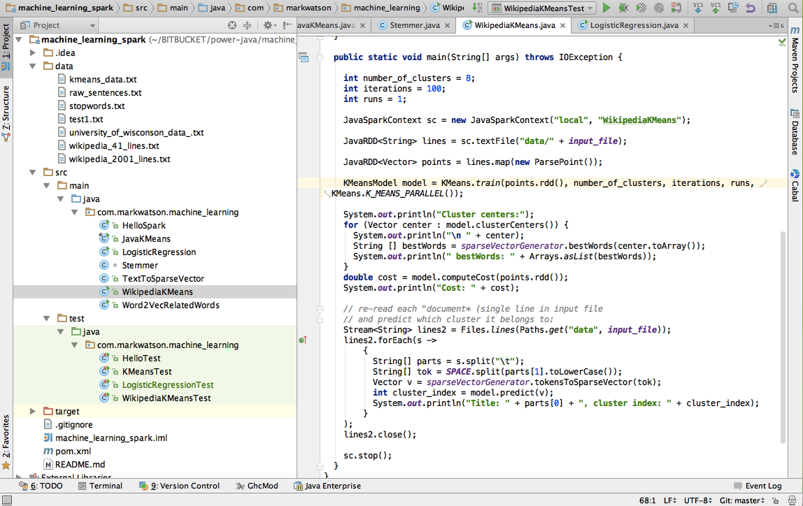
The following figure shows the project for this chapter in the Community Edition of IntelliJ:
Hello Spark - a Word Count Example
The word count example is frequently used to introduce map reduce and I will also use it here for a “hello world” type simple Spark example. In the following listing, lines 3 through 6 import the required classes. In lines 3 and 4 “RDD” stands for Resilient Distributed Datasets (RDD). Spark was written in Scala so we will sometimes see Java wrapper classes that are recognizable with the prefix “Java.” Each RDD is a collection of objects of some type that can be distributed across multiple servers in a Spark cluster. RDDs are fault tolerant and there is sufficient information in a Spark cluster to recreate any lost data due to a server or software failure.
 1 package com.markwatson.machine_learning;
 2
 3 import org.apache.spark.api.java.JavaPairRDD;
 4 import org.apache.spark.api.java.JavaRDD;
 5 import org.apache.spark.api.java.JavaSparkContext;
 6 import scala.Tuple2;
 7
 8 import java.util.Arrays;
 9 import java.util.List;
10 import java.util.Map;
11
12 public class HelloSpark {
13
14   static private List<String> tokenize(String s) {
15     return Arrays.asList(s.replaceAll("\\.", " \\. ").replaceAll(",", " , ")
16         .replaceAll(";", " ; ").split(" "));
17   }
18
19   static public void main(String[] args) {
20     JavaSparkContext sc = new JavaSparkContext("local", "Hello Spark");
21
22     JavaRDD<String> lines = sc.textFile("data/test1.txt");
23     JavaRDD<String> tokens = lines.flatMap(line -> tokenize(line));
24     JavaPairRDD<String, Integer> counts =
25         tokens.mapToPair(token ->
26 			 new Tuple2<String, Integer>(token.toLowerCase(), 1))
27               .reduceByKey((count1, count2) -> count1 + count2);
28     Map countMap = counts.collectAsMap();
29     System.out.println(countMap);
30     List<Tuple2<String, Integer>> collection = counts.collect();
31     System.out.println(collection);
32   }
33 }
Lines 14 through 17 define the simple tokenizer method that takes English text and maps it to a list of strings. I broke this out into a separate method as a reminder that punctuation needs to be handled and breaking it in to a separate method makes it easier for you to experiment with custom tokenization that might be needed for your particular text input files. One possibility is using the OpenNLP tokenizer model that we used in the last chapter. For example, we would want the string “tree.” to be tokenized as [“tree”, “.”] and not [“tree.”]. This method is used in line 23 and is called for each line in the input text file.
In this example in line 22 we are reading a local text file “data/test1.txt” but in general the argument to JavaSparkContext.textFile() can be a URI specifying a file on a local Hadoop file system (HDFS), an Amazon S3 object, of a Cassandra file system. Pay some attention to the type of the variable lines defined in line 22: the type JavaRDD<String> specifies an RDD collection where the distributed objects are strings.
The code in lines 29 through 32 is really not very complicated if we parse it out a bit at a time. The type of counts is a RDD distributed collection where each object in the collection is a pair of string and integer values. The code in lines 25 through 27 takes each token in the original text file and produces a pair (or Tuple2) values consisting of the token string and the integer 1. As an example, an array of three tokens like:
1 ["the", "dog", "ran"]
would be converted to an array of three pairs like:
1 [["the", 1], ["dog", 1], ["ran", 1]]
The statement in line 28 is uses the method reduceByKey which partitions the array of pairs by unique key value (the key being the first element in each pair) and sums the values for each matching key. The rest of this example shows two ways to extract data from an distributed RDD collection back to a Java process as local data. In line 29 we are pulling the collection of word counts into a Java Map<String,Integer> collection and in line 31 we are doing the same thing but pulling data into a list of Scala tuples. Here is what the output of the program looks like:
1     {dog=2, most=1, of=1, down=1, rabbit=1, slept=1, .=2, the=5, street=1,
2      chased=1, day=1}
3     [(most,1), (down,1), (.,2), (street,1), (day,1), (chased,1), (dog,2),
4      (rabbit,1), (of,1), (slept,1), (the,5)]
Introducing the Spark MLlib Machine Learning Library
As I update this Chapter in the spring of 2016, the Spark MLlib library is at version 2.0. I will update the git repository for this book periodically and I will try to keep the code examples compatible with the current stable versions of Spark and MLlib.
The examples in the following sections show how to apply the MLlib library to problems of logistic regression, using the K-Means algoirthm to cluster similar documents, and using the word2vec algorithm to find strong associations between words in documents.
MLlib Logistic Regression Example Using University of Wisconsin Cancer Database
We will use supervised learning in this section to build a regresion model that maps a numeric feature vector of symptoms to a numeric value where larger values close to one indicate malignancy and smaller values closer to zero indicate benign.
MLlib supports three types of linear models: Support Vector Machine (SVM), logistic regression (models for membership in one or more classes or categories), and linear regression (models that model outputs for a class as a floating point number in the range [0..1]). The Spark MLlib documentation (http://spark.apache.org/docs/latest/mllib-linear-methods.html) on these three linear models is very good and their sample programs are similar so it is easy enough to switch the type of linear model that you use.
We will use logistic regression for the example in this section. Andrew Ng, in his excellent Machine Learning class said that the first model he tries when starting a new problem is a linear model. We will repeat this example in the next section using SVM instead of logistic regression.
If you read my book Build Intelligent Systems with Javascript the training and test dataset used in this section will look familiar: University of Wisconsin breast cancer data set.
From the University of Wisconsin web page, here are the attributes with their allowed ranges in this data set:
The file data/university_of_wisconson_data_.txt contains raw data. We will use this sample data set with two changes: we clean it by removing the sample code column and the next 9 values are scaled to the range [0..1] and the class is mapped to 0 (benign) or 1 (malignant). So, our input features are scaled (values between [0 and 1] numerical values indicating clump thickness, uniformity of cell size, etc. The label that specifies what the desired prediction is the class (2 for for benign, 4 for malignant which we scale to 0 or 1)). In the following listing data is read from the training file and scaled in lines 27 through 44. Here I am using some utility methods provided by MLlib. In line 28 I am using the method JavaSparkContext.textFile to read the text file into what is effectively a list of strings (one string per input line). Lines 29 through 44 is creating a list of instances of the class LabeledPoint which contains a training label with associated numeric feature data. The container class JavaRDD acts as a list of elements that can be automatically managed across a Spark server cluster. When in development mode with a local JavaSparkContext everything is running in a single JVM so an instance of class JavaRDD behaves a lot like a simple in-memory list.
 1 package com.markwatson.machine_learning;
 2
 3 import org.apache.spark.api.java.JavaDoubleRDD;
 4 import org.apache.spark.api.java.JavaRDD;
 5 import org.apache.spark.api.java.JavaSparkContext;
 6 import org.apache.spark.api.java.function.Function;
 7 import org.apache.spark.mllib.linalg.Vectors;
 8 import org.apache.spark.mllib.regression.LabeledPoint;
 9 import org.apache.spark.mllib.regression.LinearRegressionModel;
10 import org.apache.spark.mllib.regression.LinearRegressionWithSGD;
11 import scala.Tuple2;
12
13 public class LogisticRegression {
14
15   public static double testModel(LinearRegressionModel model,
16                                  double [] features) {
17     org.apache.spark.mllib.linalg.Vector inputs = Vectors.dense(features);
18     return model.predict(inputs);
19   }
20
21   public static void main(String[] args) {
22     JavaSparkContext sc =
23 	  new JavaSparkContext("local",
24 	                       "University of Wisconson Cancer Data");
25
26     // Load and parse the data
27     String path = "data/university_of_wisconson_data_.txt";
28     JavaRDD<String> data = sc.textFile(path);
29     JavaRDD<LabeledPoint> parsedData = data.map(
30         new Function<String, LabeledPoint>() {
31           public LabeledPoint call(String line) {
32             String[] features = line.split(",");
33             double label = 0;
34             double[] v = new double[features.length - 2];
35             for (int i = 0; i < features.length - 2; i++)
36               v[i] = Double.parseDouble(features[i + 1]) * 0.09;
37             if (features[10].equals("2"))
38               label = 0; // benign
39             else
40               label = 1; // malignant
41             return new LabeledPoint(label, Vectors.dense(v));
42           }
43         }
44     );
45     // Split initial RDD into two data sets with 70% training data
46     // and 30% testing data (13L is a random seed):
47     JavaRDD<LabeledPoint>[] splits =
48 	  parsedData.randomSplit(new double[]{0.7, 0.3}, 13L);
49     JavaRDD<LabeledPoint> training = splits[0].cache();
50     JavaRDD<LabeledPoint> testing = splits[1];
51     training.cache();
52
53     // Building the model
54     int numIterations = 100;
55     final LinearRegressionModel model =
56         LinearRegressionWithSGD.train(JavaRDD.toRDD(training),
57 		                              numIterations);
58
59     // Evaluate model on training examples and compute training error
60     JavaRDD<Tuple2<Double, Double>> valuesAndPreds = testing.map(
61         new Function<LabeledPoint, Tuple2<Double, Double>>() {
62           public Tuple2<Double, Double> call(LabeledPoint point) {
63             double prediction = model.predict(point.features());
64             return new Tuple2<Double, Double>(prediction, point.label());
65           }
66         }
67     );
68     double MSE = new JavaDoubleRDD(valuesAndPreds.map(
69         new Function<Tuple2<Double, Double>, Object>() {
70           public Object call(Tuple2<Double, Double> pair) {
71             return Math.pow(pair._1() - pair._2(), 2.0);
72           }
73         }
74     ).rdd()).mean();
75     System.out.println("training Mean Squared Error = " + MSE);
76
77     // Save and load model and test:
78     model.save(sc.sc(), "generated_models");
79     LinearRegressionModel loaded_model =
80 	  LinearRegressionModel.load(sc.sc(), "generated_models");
81     double[] malignant_test_data_1 =
82 	  {0.81, 0.6, 0.92, 0.8, 0.55, 0.83, 0.88, 0.71, 0.81};
83     System.err.println("Should be malignant: " +
84 	                    testModel(loaded_model, malignant_test_data_1));
85     double[] benign_test_data_1 =
86 	  {0.55, 0.25, 0.34, 0.31, 0.29, 0.016, 0.51, 0.01, 0.05};
87     System.err.println("Should be benign (close to 0.0): " +
88                        testModel(loaded_model, benign_test_data_1));
89   }
90 }
Once the data is read and converted to numeric features the next thing we do is to randomly split the data in the input data file into two separate sets: one for training and one for testing our model after training. This data splitting is done in lines 47 and 48. Line 49 copies the training data and requests to the current Spark context to try to keep this data cached in memory. In line 50 we copy the testing data but don’t specify that the test data needs to be cached in memory.
There are two sections of code left to discuss. In lines 53 through 75 I am training the model, saving the model to disk, and testing the model while it is still in memory. In lines 77 through 89 I am reloading the saved model from disk and showing how to use it with two new numeric test vectors. This last bit of code is meant as a demonstration of embedding a model in Java code and using it.
The following three lines of code are the output of this example program. The first line of output indicates that the error for training the model is low. The last two lines show the output from reloading the model from disk and using it to evaluate two new numeric feature vectors:
This example shows a common pattern: reading training data from disk, scaling it, and building a model that is saved to disk for later use. This program can almost be reused as-is for new types of training data. You should just have to modify lines 27 through 44.
MLlib SVM Classification Example Using University of Wisconsin Cancer Database
The example in this section is very similar to that in the last section. The only differences are using the MLlib class SvmClassifier instead of the class LogisticRegression that we used in the last section and setting the number of training iterations to 500. We are using the same University of Wisconsin cancer data set in this section - refer to the previous section for a discusion of this data set.
Since the code for this section is very similar to the last example I will not list it. Please refer to the source file SvmClassifier.java and the test file SvmClassifier.java in the github repository for this book. In the repository subdirectory machine_learning_spark you will need to remove the model files generated when running the example in the previous section before running this example:
The output for this example will look like:
Note that the test data mean square error is larger than the value of 0.050140726106582885 that we obtained using logistic regression in the last section.
MLlib K-Means Example Program
We will use unsupervised learning in this section, specifically the K-Means clustering algorithm. This clustering process partitions inputs into groups that share common features. Later in this chapter we will look at an example where our input will be some randomly chosen Wikipedia articles.
K-Means analysis is useful for many types of data where you might want to cluster members of some set into different sub-groups. As an example, you might be a biologist studying fish. For each species of fish you might have attributes like length, weight, location, fresh/salt water, etc. You can use K-Means to divide fish specifies into similar sub-groups.
If your job deals with marketing to people on social media, you might want to cluster people (based on what attributes you have for users of social media) into sub-groups. If you have sparse data on some users, you might be able to infer missing data on other users.
The simple example in this section uses numeric feature vectors. Keep in mind, however our goal of processing Wikipedia text in a later section. In the next section we will see how to convert text to feature vectors, and finally, in the section after that we will cluster Wikipedia articles.
Implementing K-Means is simple but using the MLlib implementation has the advantage of being able to process very large data sets. The first step in calculating K-Means is choosing the number of desired clusters NC. The calculate NC cluster centers randomly. We then perform an inner loop until either cluster centers stop changing or a specified number of iteractions is done:
- For each data point, assign it to the cluster center closest to it.
- for each cluster center, move the center to the average location of the data points in that cluster
In practice you will repeat this clustering process many times and use the cluster centers with the minimum distortion. The distortion is the sum of the squares of the distances from each data point in a cluster to the final cluster center.
So before we look at the Wikipedia example (clustering Wikipedia articles) later in this chapter, I want to first review the JavaKMeansExample.java example from the Spark MLlib examples directory to see how to perform K-Means clustering on sample data (from the Spark source code distribution):
This is a very simple example that already uses numeric data. I copied the JavaKMeansExample.java file (changing the package name) to the github repository for his book.
The most important thing in this section that you need to learn is the required types of input data: vectors of double size floating point numbers. Each sample of data needs to be converted to a numeric feature vector. For some applications this is easy. As a hypothetical example, you might have a set of features that measure weather in your town: low temperature, high temperature, average temperature, percentage of sunshine during the day, and wind speed. All of these features are numeric and can be used as a feature vector as-is. You might have 365 samples for a given year and would like to cluster the data to see which days are similar to each other.
What if in this hypothetical example one of the features was a string representing the month? One obvious way to convert the data would be to map “January” to 1, “February” to 2, etc. We will see in the next section when we cluster Wikipedia articles that converting data to a numeric feature vector is not always so easy.
We will use the tiny sample data set provided with the MLlib KMeans example:
Here we have 6 samples and each sample has 3 features. From inspection, it looks like there are two clusters of data: the first three rows are in one cluster and the last three rows are in a second cluster. The order that feature vectors are processed in is not important; the samples in this file are organized so you can easily see the two clusters. When we run this sample program asking for two clusters we get:
We will go through the code in the sample program since it is the same general pattern we use throughout the rest of this chapter. Here is a slightly modified version of JavaKMeans.java with a few small changes from the version in the MLLib examples directory:
 1 public final class JavaKMeans {
 2
 3   private static class ParsePoint implements Function<String, Vector> {
 4     private static final Pattern SPACE = Pattern.compile(" ");
 5
 6     @Override
 7     public Vector call(String line) {
 8       String[] tok = SPACE.split(line);
 9       double[] point = new double[tok.length];
10       for (int i = 0; i < tok.length; ++i) {
11         point[i] = Double.parseDouble(tok[i]);
12       }
13       return Vectors.dense(point);
14     }
15   }
16
17   public static void main(String[] args) {
18
19     String inputFile = "data/kmeans_data.txt";
20     int k = 2; // two clusters
21     int iterations = 10;
22     int runs = 1;
23
24     JavaSparkContext sc = new JavaSparkContext("local", "JavaKMeans");
25     JavaRDD<String> lines = sc.textFile(inputFile);
26
27     JavaRDD<Vector> points = lines.map(new ParsePoint());
28
29     KMeansModel model = KMeans.train(points.rdd(), k, iterations, runs,
30 	                                 KMeans.K_MEANS_PARALLEL());
31
32     System.out.println("Cluster centers:");
33     for (Vector center : model.clusterCenters()) {
34       System.out.println(" " + center);
35     }
36     double cost = model.computeCost(points.rdd());
37     System.out.println("Cost: " + cost);
38
39     sc.stop();
40   }
41 }
The inner class ParsePoint is used to generate a single numeric feature vector given input data. In this simple case the input data is a string like “9.1 9.1 9.1” that needs to be tokenized and each token converted to a double floating point number. This inner class in the Wikipedia example will be much more complex.
In line 24 we are creating a Spark execution context. In all of the examples in this chapter we use a “local” context which means that Spark will run inside the same JVM as our example code. In production the Spark context could access a Spark cluster utilizing multiple servers.
Lines 25 and 27 introduce the use of the class JavaRDD which is the Java version of the Scala Ricj Data Definition class used internally to implement Spark. This data class can live inside a single JVM when we use a local Spark context or be spread over many servers when using a Spark server cluster. In line 25 we are reading the input strings and in line 27 we are using the inner class ParsePoint to convert the input text lines to numeric feature vectors.
Lines 29 and 30 use the static method KMeans.train to create a trained clustering model. Lines 33 through 35 print out the clusers (listing of the output was shown earlier in this section).
This simple example along with the “Hello Spark” example in the last section has shown you how to run Spark on your laptop in developers mode. In the next section we will see how to convert input text into a numeric feature vector.
Converting Text to Numeric Feature Vectors
In this section I develop a utility class TextToSparseVector that converts a set of text documents into sparse numeric feature vectors. Spark provides dense vector classes (like an array) and sparse vector classes that contain index and value pairs. For text feature vectors, In this example we will have a unique feature ID for each unique word stem (or word root) in all of the combined input documents.
We start by reading in all of the input text and forming a Map where the keys are word stems and the values are unique IDs. Any given index document will be represented with a psarse vector. For each word, the word’s stem is represented by a unique ID. The vector element at the integer ID value is set. A short document with 100 unique words would have 100 elements of the sparse vector set.
Listing of the class TextToSparseVector:
  1 package com.markwatson.machine_learning;
  2
  3 import java.nio.file.Files;
  4 import java.nio.file.Paths;
  5 import java.util.*;
  6 import java.util.stream.Stream;
  7 import org.apache.spark.mllib.linalg.Vector;
  8 import org.apache.spark.mllib.linalg.Vectors;
  9
 10 /**
 11  * Copyright Mark Watson 2015. Apache 2 license.
 12  */
 13 public class TextToSparseVector {
 14
 15   // The following value might have to be increased
 16   // for large input texts:
 17   static private int MAX_WORDS = 60000;
 18
 19   static private Set<String> noiseWords = new HashSet<>();
 20   static {
 21     try {
 22       Stream<String> lines =
 23 	    Files.lines(Paths.get("data", "stopwords.txt"));
 24       lines.forEach(s ->
 25           noiseWords.add(s)
 26       );
 27       lines.close();
 28     } catch (Exception e) { System.err.println(e); }
 29   }
 30
 31   private Map<String,Integer> wordMap = new HashMap<>();
 32   private int startingWordIndex = 0;
 33   private Map<Integer,String> reverseMap = null;
 34
 35   public Vector tokensToSparseVector(String[] tokens) {
 36     List<Integer> indices = new ArrayList();
 37     for (String token : tokens) {
 38       String stem = Stemmer.stemWord(token);
 39       if(! noiseWords.contains(stem) && validWord((stem))) {
 40         if (! wordMap.containsKey(stem)) {
 41           wordMap.put(stem, startingWordIndex++);
 42         }
 43         indices.add(wordMap.get(stem));
 44       }
 45     }
 46     int[] ind = new int[MAX_WORDS];
 47
 48     double [] vals = new double[MAX_WORDS];
 49     for (int i=0, len=indices.size(); i<len; i++) {
 50       int index = indices.get(i);
 51       ind[i] = index;
 52       vals[i] = 1d;
 53     }
 54     Vector ret = Vectors.sparse(MAX_WORDS, ind, vals);
 55     return ret;
 56   }
 57
 58   public boolean validWord(String token) {
 59     if (token.length() < 3)  return false;
 60     char[] chars = token.toCharArray();
 61     for (char c : chars) {
 62       if(!Character.isLetter(c)) return false;
 63     }
 64     return true;
 65   }
 66
 67   private static int NUM_BEST_WORDS = 20;
 68
 69   public String [] bestWords(double [] cluster) {
 70     int [] best = maxKIndex(cluster, NUM_BEST_WORDS);
 71     String [] ret = new String[NUM_BEST_WORDS];
 72     if (null == reverseMap) {
 73       reverseMap = new HashMap<>();
 74       for(Map.Entry<String,Integer> entry : wordMap.entrySet()){
 75         reverseMap.put(entry.getValue(), entry.getKey());
 76       }
 77     }
 78     for (int i=0; i<NUM_BEST_WORDS; i++)
 79 	  ret[i] = reverseMap.get(best[i]);
 80     return ret;
 81   }
 82   // following method found on Stack Overflow
 83   // and was written by user3879337. Thanks!
 84   private  int[] maxKIndex(double[] array, int top_k) {
 85     double[] max = new double[top_k];
 86     int[] maxIndex = new int[top_k];
 87     Arrays.fill(max, Double.NEGATIVE_INFINITY);
 88     Arrays.fill(maxIndex, -1);
 89
 90     top: for(int i = 0; i < array.length; i++) {
 91       for(int j = 0; j < top_k; j++) {
 92         if(array[i] > max[j]) {
 93           for(int x = top_k - 1; x > j; x--) {
 94             maxIndex[x] = maxIndex[x-1]; max[x] = max[x-1];
 95           }
 96           maxIndex[j] = i; max[j] = array[i];
 97           continue top;
 98         }
 99       }
100     }
101     return maxIndex;
102   }
103 }
The public method String [] bestWords(double [] cluster) is used for display purposes: it will be interesting to see the words in a document which provided the most evidence for its inclusion in a cluster. This Java class will be used in the next section to cluster similar Wikipedia articles.
Using K-Means to Cluster Wikipedia Articles
The Wikipedia article training files contain one article per line with the article title appearing at the beginning of the line. I have already performed some data cleaning: capturing HTML, stripping HTML tags, yielding plain text for the articles and then organizing the data one article per line in the input text file. I am providing two input files: one containing 41 articles and one containing 2001 articles.
One challenge we face is converting the text of an article into a numeric feature vector. This was easy to do in an earlier section using cancer data already in numeric form; I just had to discard one data attribute and scale the remaining data atrributes.
In addition to converting input data into numeric feature vectors we also need to decide how many clusters we want the K-Means algorithm to partitian our data into.
Given the class TextToSparseVector developed in the last section, the code to cluster Wikipedia articles is fairly straightforward. In the following listing of the class WikipediaKMeans
 1 // This example is derived from the Spark MLlib examples
 2
 3 package com.markwatson.machine_learning;
 4
 5 import java.io.IOException;
 6 import java.nio.file.Files;
 7 import java.nio.file.Paths;
 8 import java.util.Arrays;
 9 import java.util.regex.Pattern;
10 import java.util.stream.Stream;
11
12 import org.apache.spark.SparkConf;
13 import org.apache.spark.api.java.JavaRDD;
14 import org.apache.spark.api.java.JavaSparkContext;
15 import org.apache.spark.api.java.function.Function;
16
17 import org.apache.spark.mllib.clustering.KMeans;
18 import org.apache.spark.mllib.clustering.KMeansModel;
19 import org.apache.spark.mllib.linalg.Vector;
20 import org.apache.spark.mllib.linalg.Vectors;
21
22 public class WikipediaKMeans {
23
24   // there are two example files in ./data/: one with
25   // 41 articles and one with 2001
26   //private final static String input_file = "wikipedia_41_lines.txt";
27   private final static String input_file = "wikipedia_2001_lines.txt";
28
29   private static TextToSparseVector sparseVectorGenerator =
30    new TextToSparseVector();
31   private static final Pattern SPACE = Pattern.compile(" ");
32
33   private static class ParsePoint implements Function<String, Vector> {
34
35     @Override
36     public Vector call(String line) {
37       String[] tok = SPACE.split(line.toLowerCase());
38       return sparseVectorGenerator.tokensToSparseVector(tok);
39     }
40   }
41
42   public static void main(String[] args) throws IOException {
43
44     int number_of_clusters = 8;
45     int iterations = 100;
46     int runs = 1;
47
48     JavaSparkContext sc = new JavaSparkContext("local", "WikipediaKMeans");
49     JavaRDD<String> lines = sc.textFile("data/" + input_file);
50     JavaRDD<Vector> points = lines.map(new ParsePoint());
51     KMeansModel model = KMeans.train(points.rdd(), number_of_clusters,
52 	                                 iterations, runs,
53                                      KMeans.K_MEANS_PARALLEL());
54
55     System.out.println("Cluster centers:");
56     for (Vector center : model.clusterCenters()) {
57       System.out.println("\n " + center);
58       String [] bestWords = sparseVectorGenerator.bestWords(center.toArray());
59       System.out.println(" bestWords: " + Arrays.asList(bestWords));
60     }
61     double cost = model.computeCost(points.rdd());
62     System.out.println("Cost: " + cost);
63
64     // re-read each "document* (single line in input file
65     // and predict which cluster it belongs to:
66     Stream<String> lines2 = Files.lines(Paths.get("data", input_file));
67     lines2.forEach(s ->
68         {
69           String[] parts = s.split("\t");
70           String[] tok = SPACE.split(parts[1].toLowerCase());
71           Vector v = sparseVectorGenerator.tokensToSparseVector(tok);
72           int cluster_index = model.predict(v);
73           System.out.println("Title: " + parts[0] + ", cluster index: " +
74 		                     cluster_index);
75         }
76     );
77     lines2.close();
78
79     sc.stop();
80   }
81 }
The class WikipediaKMeans is fairly simple because most of the work is done converting text to feature vectors using class TextToSparseVector that we saw in the last seciton. The Spark setup code is also similar to that seen in our tiny HelloSpark example.
The parsepoint method defined in lines 33 to 40 uses the method tokensToSparseVector (defined in class TextToSparseVector) to convert the text in one line of the input file (remember that each line contains text for an entire Wikipedia article) to a sparse feature vector. There are two important parameters that you will want to experiment with. These parameters are defined on lines 44 and 45 and set the desired number of clusters and the number of iterations you want to run to form clusters. I suggest leaving iterations set initially to 100 as it is in the code and then vary number_of_clusters. If you are using this code in one of your own projects with a different data set then you might also want to experiment with running more iterations. If you cluster a very large number of text documents then you may have to increase the constant value MAX_WORDS set in line 9 in the class TextToSparseVector.
In line 48 we are creating a new Spark context that is local and will run in the same JVM as your application code. Lines 49 and 50 read in the text data from Wikipedia and create a JavaRDD of vectors pass to the K-Means clustering code that is called in lines 51 to 53.
Here are a few cluster indices for the 2001 input Wikipedia articles that are printed out by cluster index. When you run the sample program this list of documents assigned to eight different clusters is a lot of output. In the following I am listing just a small bit of the output for the first four clusters. If you look carefully at the generated clusters you will notice that Cluster seems not to be so useful since there are really two or three topics represented in the cluster. This might indicate re-running the clustering with a larger number of requested clusters (i.e., increasing the value of number_of_clusters). On the other hand, Cluster 1 seems very good, almost all articles are dealing with sports.
This example program can be reused in your applications with few changes. You will probably want to manually assign meaningful labels to each cluster index and store the label with each document. For example, the cluster at index 1 would probably be labeled as “sports.”
Using SVM for Text Classification
  1 package com.markwatson.machine_learning;
  2
  3 import org.apache.spark.api.java.JavaDoubleRDD;
  4 import org.apache.spark.api.java.JavaRDD;
  5 import org.apache.spark.api.java.JavaSparkContext;
  6 import org.apache.spark.api.java.function.Function;
  7 import org.apache.spark.mllib.classification.SVMModel;
  8 import org.apache.spark.mllib.classification.SVMWithSGD;
  9 import org.apache.spark.mllib.linalg.Vector;
 10 import org.apache.spark.mllib.regression.LabeledPoint;
 11 import scala.Tuple2;
 12
 13 import java.io.IOException;
 14 import java.nio.file.Files;
 15 import java.nio.file.Paths;
 16 import java.util.*;
 17 import java.util.regex.Pattern;
 18 import java.util.stream.Stream;
 19
 20 /**
 21  * Created by markw on 11/25/15.
 22  */
 23 public class SvmTextClassifier {
 24   private final static String input_file = "test_classification.txt";
 25
 26   private static TextToSparseVector sparseVectorGenerator = new TextToSparseVect\
 27 or();
 28   private static final Pattern SPACE = Pattern.compile(" ");
 29
 30   static private String [] tokenizeAndRemoveNoiseWords(String s) {
 31     return s.toLowerCase().replaceAll("\\.", " \\. ").replaceAll(",", " , ")
 32         .replaceAll("\\?", " ? ").replaceAll("\n", " ")
 33         .replaceAll(";", " ; ").split(" ");
 34   }
 35
 36   static private Map<String, Integer> label_to_index = new HashMap<>();
 37   static private int label_index_count = 0;
 38   static private Map<String, String> map_to_print_original_text = new HashMap<>(\
 39 );
 40
 41   private static class ParsePoint implements Function<String, LabeledPoint> {
 42
 43     @Override
 44     public LabeledPoint call(String line) {
 45       String [] data_split = line.split("\t");
 46       String label = data_split[0];
 47       Integer label_index = label_to_index.get(label);
 48       if (null == label_index) {
 49         label_index = label_index_count;
 50         label_to_index.put(label, label_index_count++);
 51       }
 52       Vector tok = sparseVectorGenerator.tokensToSparseVector(
 53                           tokenizeAndRemoveNoiseWords(data_split[1]));
 54       // Save original text, indexed by compressed features, for later
 55       // display (for debug ony):
 56       map_to_print_original_text.put(tok.compressed().toString(), line);
 57       return new LabeledPoint(label_index, tok);
 58     }
 59   }
 60
 61   public static void main(String[] args) throws IOException {
 62
 63     JavaSparkContext sc = new JavaSparkContext("local", "WikipediaKMeans");
 64
 65     JavaRDD<String> lines = sc.textFile("data/" + input_file);
 66
 67     JavaRDD<LabeledPoint> points = lines.map(new ParsePoint());
 68
 69     // Split initial RDD into two with 70% training data and 30% testing
 70     // data (13L is a random seed):
 71     JavaRDD<LabeledPoint>[] splits =
 72        points.randomSplit(new double[]{0.7, 0.3}, 13L);
 73     JavaRDD<LabeledPoint> training = splits[0].cache();
 74     JavaRDD<LabeledPoint> testing = splits[1];
 75     training.cache();
 76
 77     // Building the model
 78     int numIterations = 500;
 79     final SVMModel model =
 80         SVMWithSGD.train(JavaRDD.toRDD(training), numIterations);
 81     model.clearThreshold();
 82     // Evaluate model on testing examples and compute training error
 83     JavaRDD<Tuple2<Double, Double>> valuesAndPreds = testing.map(
 84         new Function<LabeledPoint, Tuple2<Double, Double>>() {
 85           public Tuple2<Double, Double> call(LabeledPoint point) {
 86             double prediction = model.predict(point.features());
 87             System.out.println(" ++ prediction: " + prediction + " original: " +
 88               map_to_print_original_text.get(
 89                     point.features().compressed().toString()));
 90             return new Tuple2<Double, Double>(prediction, point.label());
 91           }
 92         }
 93     );
 94
 95     double MSE = new JavaDoubleRDD(valuesAndPreds.map(
 96         new Function<Tuple2<Double, Double>, Object>() {
 97           public Object call(Tuple2<Double, Double> pair) {
 98             return Math.pow(pair._1() - pair._2(), 2.0);
 99           }
100         }
101     ).rdd()).mean();
102     System.out.println("Test Data Mean Squared Error = " + MSE);
103
104     sc.stop();
105   }
106
107   static private Set<String> noiseWords = new HashSet<>();
108   static {
109     try {
110       Stream<String> lines = Files.lines(Paths.get("data", "stopwords.txt"));
111       lines.forEach(s -> noiseWords.add(s));
112       lines.close();
113     } catch (Exception e) { System.err.println(e); }
114   }
115
116 }
This code calculates prediction values less than zero for the EDUCATION class and greater than zero for the HEALTH class:
Using word2vec To Find Similar Words In Documents
Google released their open source word2vec library as Apache 2 licensed open source. The Deeplearning4j project and Spark’s MLlib both contain implementations. As I write this chapter the Deeplearning4j version has more flexibility but we will use the MLlib version here. We cover Deeplearning4j in a later chapter. We will use the sample data file from the Deeplearning4j project in this section.
The word2vec library can identify which other words in text are strongly related to any other word in the text. If you run word2vec on a large sample of English language text you will find the the word woman is closely associated with the word man, the word child to the word mother, the word road to the word car, etc.
The following listing shows the class Word2VecRelatedWords that is fairly simple because all we need to do is tokenize text, discard noise (or stop) words, and convert the input text to the correct Spark data types for processing by the MLlib class *Word2VecModel**.
 1 package com.markwatson.machine_learning;
 2
 3 import org.apache.spark.api.java.JavaRDD;
 4 import org.apache.spark.api.java.JavaSparkContext;
 5 import org.apache.spark.mllib.feature.Word2Vec;
 6 import org.apache.spark.mllib.feature.Word2VecModel;
 7
 8 import java.io.IOException;
 9 import java.nio.file.Files;
10 import java.nio.file.Paths;
11 import java.util.*;
12 import java.util.stream.Collectors;
13 import java.util.stream.Stream;
14
15 import scala.Tuple2;
16
17 public class Word2VecRelatedWords {
18   // Use the example data file form the deeplearning4j.org word2vec example:
19   private final static String input_file = "data/raw_sentences.txt";
20
21   static private List<String> tokenizeAndRemoveNoiseWords(String s) {
22     return Arrays.asList(s.toLowerCase().replaceAll("\\.", " \\. ")
23         .replaceAll(",", " , ").replaceAll("\\?", " ? ")
24         .replaceAll("\n", " ").replaceAll(";", " ; ").split(" "))
25         .stream().filter((w) ->
26 		     ! noiseWords.contains(w)).collect(Collectors.toList());
27   }
28
29   public static void main(String[] args) throws IOException {
30     JavaSparkContext sc = new JavaSparkContext("local", "WikipediaKMeans");
31
32     String sentence = new String(Files.readAllBytes(Paths.get(input_file)));
33     List<String> words = tokenizeAndRemoveNoiseWords(sentence);
34     List<List<String>> localWords = Arrays.asList(words, words);
35     Word2Vec word2vec = new Word2Vec().setVectorSize(10).setSeed(113L);
36     JavaRDD<List<String>> rdd_word_list = sc.parallelize(localWords);
37     Word2VecModel model = word2vec.fit(rdd_word_list);
38
39     Tuple2<String, Object>[] synonyms = model.findSynonyms("day", 15);
40     for (Object obj : synonyms)
41 	  System.err.println("-- words associated with day: " + obj);
42
43     synonyms = model.findSynonyms("children", 15);
44     for (Object obj : synonyms)
45 	  System.err.println("-- words associated with children: " + obj);
46
47     synonyms = model.findSynonyms("people", 15);
48     for (Object obj : synonyms)
49 	  System.err.println("-- words associated with people: " + obj);
50
51     synonyms = model.findSynonyms("three", 15);
52     for (Object obj : synonyms)
53 	  System.err.println("-- words associated with three: " + obj);
54
55     synonyms = model.findSynonyms("man", 15);
56     for (Object obj : synonyms)
57 	  System.err.println("-- words associated with man: " + obj);
58
59     synonyms = model.findSynonyms("women", 15);
60     for (Object obj : synonyms)
61 	  System.err.println("-- words associated with women: " + obj);
62
63     sc.stop();
64   }
65
66   static private Set<String> noiseWords = new HashSet<>();
67   static {
68     try {
69       Stream<String> lines = Files.lines(Paths.get("data", "stopwords.txt"));
70       lines.forEach(s -> noiseWords.add(s));
71       lines.close();
72     } catch (Exception e) { System.err.println(e); }
73   }
74 }
The output from this example program is:
While word2vec results are just the result of statistical processing and the code does not understand the semantic of the English language, the results are still impressive.
Chapter Wrap Up
In the previous chapter we used machine learning for natural language processing using the OpenNLP project. In the examples in this chapter we used the Spark MLlib library for for logistic regression, document clustering, and determining which words are closely associated with each other.
You can go far using OpenNLP and Spark MLlib in your projects. There are a few things to keep in mind, however. One of the most difficult aspects of machine learning is finding and preparing training data. This process will be very dependant on what kind of project you are working on and what sources of data you have.
One of the most powerful machine learning techniques is artificial neural networks. I have a long history of using neural networks (I was on a DARPA neural network advisory panel and wrote the first version of the commercial ANSim neural network product in the late 1980s). I decided not to cover simple neural network models in this book because I have already written about neural networks in one chapter of my book Practical Artificial Intelligence Programming in Java. “Deep learning” neural networks are also very effective (if difficult to use) for some types of machine learning problems (e.g., image recognition and speech recognition) and we will use the Deeplearning4j project in a later chapter.
In the next chapter we cover another type of machine learning: anomaly detection.