Deep Learning Using Deeplearning4j
The Deeplearning4j.org Java library supports several neural network algorithms including support for Deep Learning (DL). We will look at an example of DL implementing Deep-Belief networks using the same University of Wisconsin cancer database that we used in the chapters on machine learning with Spark and on anomaly detection. Deep learning refers to neural networks with many layers, possibly with weights connecting neurons in non-adjacent layers which makes it possible to model temporal and spacial patterns in data.
I am going to assume that you have some knowledge of simple backpropagation neural networks. If you are unfamiliar with neural networks you might want to pause and do a web search for “neural networks backpropagation tutorial” or read the neural network chapter in my book Practical Artificial Intelligence Programming With Java, 4th edition.
The difficulty in training many layer networks with backpropagation is that the delta errors in the layers near the input layer (and far from the output layer) get very small and training can take a very long time even on modern processors and GPUs. Geoffrey Hinton and his colleagues created a new technique for pretraining weights. In 2012 I took a Coursera course taught by Hinton and some colleagues titled ‘Neural Networks for Machine Learning’ and the material may still be available online when you read this book.
For Java developers, Deeplearning4j is a great starting point for experimenting with deep learning. If you also use Python then there are good tutorials and other learning assets at deeplearning.net.
Deep Belief Networks
Deep Belief Networks (DBN) are a type of deep neural network containing multiple hidden neuron layers where there are no connections between neurons inside any specific hidden layer. Each hidden layer learns features based on training data an the values of weights from the previous hidden layer. By previous layer I refer to the connected layer that is closer to the input layer. A DBN can learn more abstract features, with more abstraction in the hidden layers “further” from the input layer.
DBNs are first trained a layer at a time. Initially a set of training inputs is used to train the weights between the input and the first hidden layer of neurons. Technically, as we preliminarily train each succeeding pair of layers we are training a restricted Boltzmann machine (RBM) to learn a new set of features. It is enough for you to know at this point that RBMs are two layers, input and output, that are completely connected (all neurons in the first layer have a weighted connection to each neuron in the next layer) and there are no inner-layer connections.
As we progressively train a DBN, the output layer for one RBM becomes the input layer for the next neuron layer pair for preliminary training.
Once the hidden layers are all preliminarily trained then backpropagation learning is used to retrain the entire network but now delta errors are calculated by comparing the forward pass outputs with the training outputs and back-propagating errors to update weights in layers proceeding back towards the first hidden layer.
The important thing to understand is that backpropagation tends to not work well for networks with many hidden layers because the back propagated errors get smaller as we process backwards towards the input neurons - this would cause network training to be very slow. By precomputing weights using RBM pairs, we are closer to a set of weights to minimize errors over the training set (and the test set).
Deep Belief Example
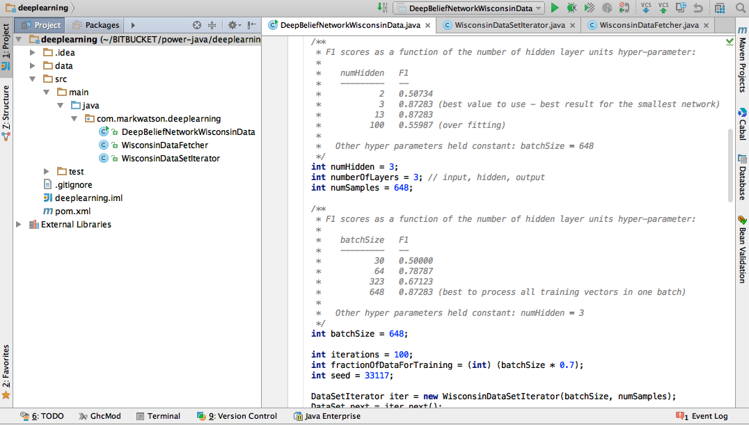
The following screen show shows an IntelliJ project (you can use the free community orprofessional version for the examples in this book) for the example in this chapter:
The Deeplearning4j library uses user-written Java classes to import training and testing data into a form that the Deeplearning4j library can use. The following listing shows the implementation of the class WisconsinDataSetIterator that iterates through the University of Wisconsin cancer data set:
 1 package com.markwatson.deeplearning;
 2
 3 import org.deeplearning4j.datasets.iterator.BaseDatasetIterator;
 4
 5 import java.io.FileNotFoundException;
 6
 7
 8 public class WisconsinDataSetIterator extends BaseDatasetIterator {
 9   private static final long serialVersionUID = -2023454995728682368L;
10
11   public WisconsinDataSetIterator(int batch, int numExamples)
12          throws FileNotFoundException {
13     super(batch, numExamples, new WisconsinDataFetcher());
14   }
15 }
The WisconsinDataSetIterator constructor calls its super class with an instance of the class WisconsinDataFetcher (defined in the next listing) to read the Comma Separated Values (CSV) spreadsheet data from the file data/cleaned_wisconsin_cancer_data.csv:
 1 package com.markwatson.deeplearning;
 2
 3 import org.deeplearning4j.datasets.fetchers.CSVDataFetcher;
 4
 5 import java.io.FileInputStream;
 6 import java.io.FileNotFoundException;
 7
 8 /**
 9  * Created by markw on 10/5/15.
10  */
11 public class WisconsinDataFetcher extends CSVDataFetcher {
12
13   public WisconsinDataFetcher() throws FileNotFoundException {
14     super(new FileInputStream("data/cleaned_wisconsin_cancer_data.csv"), 9);
15   }
16   @Override
17   public void fetch(int i) {
18     super.fetch(i);
19   }
20
21 }
In line 14, the last argument 9 defines which column in the input CSV file contains the label data. This value is zero indexed so if you look at the input file data/cleaned_wisconsin_cancer_date.csv this will be the last column. Values of 4 in the last column idicate malignant and values of 2 indicate not malignant.
The following listing shows the definition of the class DeepBeliefNetworkWisconsinData that reads the University of Wisconsin cancer data set using the code in the last two listings, randmly selects part of it to use for training and for testing, creates a DBN, and tests it. The value of the variable numHidden set in line 51 refers to the number of neurons in each hidden layer. Setting numberOfLayers to 3 in line 52 indicates that we will just use a single hidden layer since this value (3) also counts the input and output layers.
The network is configured and constructed in lines 83 through 104. If we increased the number of hidden units (something that you might do for more complex problems) then you would repeat lines 88 through 97 to add a new hidden layer, and you would change the layer indices (first argument) as appropriate in calls to the chained method .layer().
  1 package com.markwatson.deeplearning;
  2
  3 import org.deeplearning4j.datasets.iterator.DataSetIterator;
  4 import org.deeplearning4j.eval.Evaluation;
  5 import org.deeplearning4j.nn.conf.MultiLayerConfiguration;
  6 import org.deeplearning4j.nn.conf.NeuralNetConfiguration;
  7 import org.deeplearning4j.nn.conf.layers.OutputLayer;
  8 import org.deeplearning4j.nn.conf.layers.RBM;
  9 import org.deeplearning4j.nn.multilayer.MultiLayerNetwork;
 10 import org.deeplearning4j.nn.weights.WeightInit;
 11 import org.nd4j.linalg.api.ndarray.INDArray;
 12 import org.nd4j.linalg.dataset.DataSet;
 13 import org.nd4j.linalg.dataset.SplitTestAndTrain;
 14 import org.nd4j.linalg.factory.Nd4j;
 15 import org.nd4j.linalg.lossfunctions.LossFunctions;
 16 import org.slf4j.Logger;
 17 import org.slf4j.LoggerFactory;
 18
 19 import java.io.*;
 20 import java.nio.file.Files;
 21 import java.nio.file.Paths;
 22 import java.util.Random;
 23
 24 import org.apache.commons.io.FileUtils;
 25
 26 /**
 27  * Train a deep belief network on the University of Wisconsin Cancer Data Set.
 28  */
 29 public class DeepBeliefNetworkWisconsinData {
 30
 31   private static Logger log =
 32     LoggerFactory.getLogger(DeepBeliefNetworkWisconsinData.class);
 33
 34   public static void main(String[] args) throws Exception {
 35
 36     final int numInput = 9;
 37     int outputNum = 2;
 38     /**
 39      * F1 scores as a function of the number of hidden layer
 40      * units hyper-parameter:
 41      *
 42      *    numHidden   F1
 43      *    ---------   --
 44      *            2   0.50734
 45      *            3   0.87283 (value to use - best result / smallest network)
 46      *           13   0.87283
 47      *          100   0.55987 (over fitting)
 48      *
 49      *   Other hyper parameters held constant: batchSize = 648
 50      */
 51     int numHidden = 3;
 52     int numberOfLayers = 3; // input, hidden, output
 53     int numSamples = 648;
 54
 55     /**
 56      * F1 scores as a function of the number of batch size:
 57      *
 58      *    batchSize   F1
 59      *    ---------   --
 60      *           30   0.50000
 61      *           64   0.78787
 62      *          323   0.67123
 63      *          648   0.87283 (best to process all training vectors in one batch)
 64      *
 65      *   Other hyper parameters held constant: numHidden = 3
 66      */
 67     int batchSize = 648; // equal to number of samples
 68
 69     int iterations = 100;
 70     int fractionOfDataForTraining = (int) (batchSize * 0.7);
 71     int seed = 33117;
 72
 73     DataSetIterator iter = new WisconsinDataSetIterator(batchSize, numSamples);
 74     DataSet next = iter.next();
 75     next.normalizeZeroMeanZeroUnitVariance();
 76
 77     SplitTestAndTrain splitDataSets =
 78 	  next.splitTestAndTrain(fractionOfDataForTraining, new Random(seed));
 79     DataSet train = splitDataSets.getTrain();
 80     DataSet test = splitDataSets.getTest();
 81
 82     MultiLayerConfiguration conf = new NeuralNetConfiguration.Builder()
 83         .seed(seed) //use the same random seed
 84         .iterations(iterations)
 85         .l1(1e-1).regularization(true).l2(2e-4)
 86         .list(numberOfLayers - 1) // don't count the input layer
 87         .layer(0,
 88             new RBM.Builder(RBM.HiddenUnit.RECTIFIED, RBM.VisibleUnit.GAUSSIAN)
 89                 .nIn(numInput)
 90                 .nOut(numHidden)
 91                 // set variance of random initial weights based on
 92                 // input and output layer size:
 93                 .weightInit(WeightInit.XAVIER)
 94                 .dropOut(0.25)
 95                 .build()
 96         )
 97         .layer(1, new OutputLayer.Builder(LossFunctions.LossFunction.MCXENT)
 98             .nIn(numHidden)
 99             .nOut(outputNum)
100             .activation("softmax")
101             .build()
102         )
103         .build();
104     MultiLayerNetwork model = new MultiLayerNetwork(conf);
105     model.init();
106     model.fit(train);
107
108     log.info("\nEvaluating model:\n");
109     Evaluation eval = new Evaluation(outputNum);
110     INDArray output = model.output(test.getFeatureMatrix());
111
112     for (int i = 0; i < output.rows(); i++) {
113       String target = test.getLabels().getRow(i).toString();
114       String predicted = output.getRow(i).toString();
115       log.info("target: " + target + " predicted: " + predicted);
116     }
117
118     eval.eval(test.getLabels(), output);
119     log.info(eval.stats());
120
121     /**
122      * Save the model for reuse:
123      */
124     OutputStream fos = Files.newOutputStream(Paths.get("saved-model.bin"));
125     DataOutputStream dos = new DataOutputStream(fos);
126     Nd4j.write(model.params(), dos);
127     dos.flush();
128     dos.close();
129     FileUtils.writeStringToFile(
130        new File("conf.json"),
131                 model.getLayerWiseConfigurations().toJson());
132
133     /**
134      * Load saved model and test again:
135      */
136     log.info("\nLoad saved model from disk:\n");
137     MultiLayerConfiguration confFromJson =
138 	  MultiLayerConfiguration.fromJson(
139                      FileUtils.readFileToString(new File("conf.json")));
140     DataInputStream dis = new DataInputStream(
141                                 new FileInputStream("saved-model.bin"));
142     INDArray newParams = Nd4j.read(dis);
143     dis.close();
144     MultiLayerNetwork savedModel = new MultiLayerNetwork(confFromJson);
145     savedModel.init();
146     savedModel.setParameters(newParams);
147
148     log.info("\nEvaluating model loaded from disk:\n");
149     Evaluation eval2 = new Evaluation(outputNum);
150     INDArray output2 = savedModel.output(test.getFeatureMatrix());
151
152     for (int i = 0; i < output2.rows(); i++) {
153       String target = test.getLabels().getRow(i).toString();
154       String predicted = output.getRow(i).toString();
155       log.info("target: " + target + " predicted: " + predicted);
156     }
157
158     eval2.eval(test.getLabels(), output2);
159     log.info(eval2.stats());
160   }
161 }
In line 71 we set fractionOfDataForTraining to 0.7 which means that we will use 70% of the available data for training and 30% for testing. It is very important to not use training data for testing because performance on recognizing training data should always be good assuming that you have enough memory capacity in a network (i.e., enough hidden units and enough neurons in each hidden layer). In lines 78 through 81 we divide our data into training and testing disjoint sets.
In line 86 we are setting three meta learning parameters: learning rate for the first set of weights between the input and hidden layer to be 1e-1, setting the model to use regularization, and setting the learning rate for the hidden to output weights to be 2e-4.
In line 95 we are setting the dropout factor, here saying that we will randomly not use 25% of the neurons for any given training example. Along with regularization, using dropout helps prevent overfitting. Overfitting occurs when a neural netowrk fails to generalize and learns noise in training data. The goal is to learn important features that affect the utility of a trained model for processing new data. We don’t want to learn random noise in the data as important features. Another way to prevent overfitting is to use the smallest possible number of neurons in hidden labels and still perform well on the independent test data.
After training the model in lines 105 through 107, we test the model (lines 110 through 120) on the separate test data. The program output when I ran the model is:
The F1 score is calculated as twice precision times recall, all divided by precision + recall. We would like F1 to be as close to 1.0 as possible and it is common to spend a fair amount of time experimenting with meta learning paramters to increase F1.
It is also fairly common to try to learn good values of meta learning paramters also. We won’t do this here but the process involves splitting the data into three disjoint sets: training, validation, and testing. The meta parameters are varied, training is performed, and using the validation data the best set of meta parameters is selected. Finally, we test the netowrk as defined my meta parameters and learned weights for those meta parameters with the separate test data to see what the effective F1 score is.
Deep Learning Wrapup
I first used complex neural network topologies in the late 1980s for phoneme (speech) recognition, specifically using time delay neural networks and I gave a talk about it at IEEE First Annual International Conference on Neural Networks San Diego, California June 21-24, 1987. Back then, neural networks were not really considered to be a great technology for this application but in the present time Google, Microsoft, and other companies are using deep (many layered) neural networks for speech and image recognition. Exciting work is also being done in the field of natural language processing. I just provided a small example in this chapter that you can experiment with easily. I wanted to introduce you to Deeplearning4j because I think it is probably the easiest way for Java developers to get started working with many layered neural networks and I refer you to the project documentation.