
Table of Contents
- Problem 1
- Writing in Markua
-
AnaliAnálisis de cluscluster
- title: “Tarea Cluster : solucion”output:html_document:keep_md: truedf_print: pagedtheme: spacelabtoc: yeseditor_options:chunk_output_type: console
- Realiza también una gráfica que muestre todas las posibles combinaciones :
- Realiza un análisis de clúster jerárquico y selecciona cuantos clústeres posibles sé pueden formar :
- Calculo de la Matriz de Distancias Euclidianas
- Calcula el dendograma de la matriz de distancias
- Gráfica del Dendograma para k=5
- Gráfica del Dendograma para k=6
- Realiza ahora un análisis de K-means para calcular con mayor precisión el número de clúster :
- Calcular el % de cambio en las distancias
- Grafica del % vs Numero de cluster
- Concluye cuál será el número más adecuado de clúster a formar :
Problem 1
Contexto: Una fábrica produce piezas mecánicas que deben pasar por un proceso de inspección de calidad. Si una pieza no cumple con los estándares de calidad, se envía a retrabajo.
El proceso de retracodigo2ene una probabilidad de éxito, después de lo cual la pieza se vuelve a inspeccionar. Si la pieza falla nuevamente, se descarta.
Parámetros del Problema:
Tasa de producción: 10 piezas por hora.
Tiempo de inspección: 5 minutos por pieza.
Probabilidad de falla en la inspección inicial: 20%.
Tiempo de retrabajo: 15 minutos por pieza.
Probabilidad de éxito en el retrabajo: 70%.
Tiempo de inspección después del retrabajo: 5 minutos por pieza. 7.
Cantidad máxima de retrabajo: 3
Objetivo: Simular el proceso durante un turno de 8 horas para determinar:
- El número total de piezas producidas.
- El número de piezas que pasan la inspección inicial.
- El número de piezas que requieren retrabajo.
- El número de piezas que pasan la inspección después del retrabajo.
- El número de piezas descartadas.
- El tiempo total de espera en cola para retrabajo.
Pasos para la Simulación:
- Generar las piezas: Crear un evento de llegada de piezas cada 6 minutos (10 piezas por hora).
- Inspección inicial: Para cada pieza, determinar si pasa o falla la inspección inicial (20% de probabilidad de falla).
- Retrabajo: Para las piezas que fallan, enviar a retrabajo si hay capacidad disponible; si no, esperar en cola.
- Resultados: Registrar los resultados de cada inspección y retrabajo, así como el tiempo de espera en cola.
Writing in Markua
Writing in Markua is easy! You can learn most of what you need to know with just a few examples.
To make italic text you surround it with single asterisks. To make bold text you surround it with double asterisks.
Section One
You can start new sections by starting a line with two # signs and a space, and then typing your section title.
Sub-Section One
You can start new sub-sections by starting a line with three # signs and a space, and then typing your sub-section title.
Including a Chapter in the Sample Book
At the top of this file, you will also see a line at the top:
1 {sample: true}
Leanpub has the ability to make a sample book, which interested readers can download or read online. If you add this line above a chapter heading, then when you publish your book, this chapter will be included in a separate sample book for these interested readers.
Links
You can add web links easily.
Here’s a link to the Leanpub homepage.
Images
You can add an image to your book in a similar way.
First, add the image to the “Resources” folder for your book. You will find the “Resources” folder under the “Manuscript” menu to the left.
If you look in your book’s “Resources” folder right now, you will see that there is an example image there with the file name “palm-trees.jpg”. Here’s how you can add this image to your book:

If you want to add a figure title, you put it in quotes:
If you want to add descriptive alt text, which is good for accessibility, you put it between the square brackets:
You can also set the alt text and/or the figure title in an attribute list:
Finally, if no title is provided, and the alt-title document setting is the default of all, the alt text will be used as the figure title instead of as alt text.
You can set the important document settings at Settings > Generation Settings.
Lists
Numbered Lists
You make a numbered list like this:
- kale
- carrot
- ginger
Bulleted Lists
You make a bulleted list like this:
- kale
- carrot
- ginger
Definition Lists
You can even have definition lists!
- term 1
-
definition 1a
-
definition 1b
- term 2
-
definition 2
Code Samples
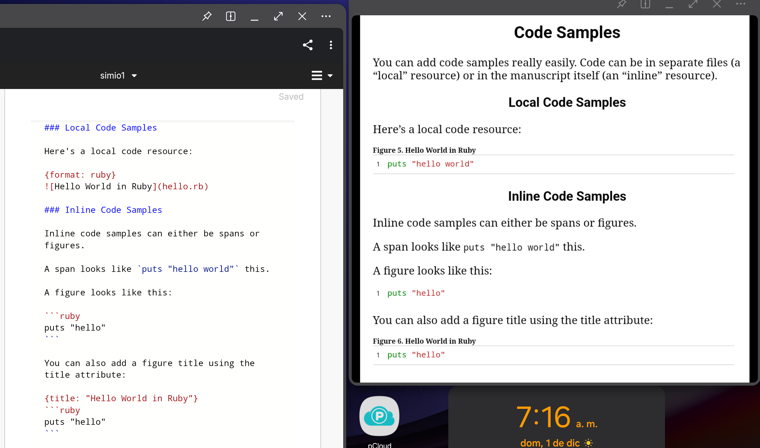
You can add code samples really easily. Code can be in separate files (a “local” resource) or in the manuscript itself (an “inline” resource).
Local Code Samples
Here’s a local code resource:
Inline Code Samples
Inline code samples can either be spans or figures.
A span looks like puts "hello world" this.
A figure looks like this:
1 puts "hello"
You can also add a figure title using the title attribute:
1 puts "hello"
Tables
You can insert tables easily inline, using the GitHub Flavored Markdown (GFM) table syntax:
| Header 1 | Header 2 |
|---|---|
| Content 1 | Content 2 |
| Content 3 | Content 4 Can be Different Length |
Tables work best for numeric tabular data involving a small number of columns containing small numbers:
| Central Bank | Rate |
|---|---|
| JPY | -0.10% |
| EUR | 0.00% |
| USD | 0.00% |
| CAD | 0.25% |
Definition lists are preferred to tables for most use cases, since reading a large table with many columns is terrible on phones and since typing text in a table quickly gets annoying.
Math
You can easily insert math equations inline using either spans or figures.
Here’s one of the kinematic equations  inserted as a span inside a sentence.
Here’s some math inserted as a figure.
Headings
Markua supports both of Markdown’s heading styles.
The preferred style, called atx headers, has the following meaning in Markua:
 1 {class: part}
 2 # Part
 3
 4 This is a paragraph.
 5
 6 # Chapter
 7
 8 This is a paragraph.
 9
10 ## Section
11
12 This is a paragraph.
13
14 ### Sub-section
15
16 This is a paragraph.
17
18 #### Sub-sub-section
19
20 This is a paragraph.
21
22 ##### Sub-sub-sub-section
23
24 This is a paragraph.
25
26 ###### Sub-sub-sub-sub-section
27
28 This is a paragraph.
Note the use of three backticks in the above example, to treat the Markua like inline code (instead of actually like headers).
The other style of headers, called Setext headers, has the following headings:
 1 {class: part}
 2 Part
 3 ====
 4
 5 This is a paragraph.
 6
 7 Chapter
 8 =======
 9
10 This is a paragraph.
11
12 Section
13 -------
14
15 This is a paragraph.
Setext headers look nice, but only if you’re only using chapters and sections.
If you want to add sub-sections (or lower), you’ll be using atx headers for at
least some of your headers. My advice is to just use atx headers all the time.
(The {class: part} attribute list on a chapter header to make a part header
does actually work with Setext headers, but it’s really ugly.)
Note that while it is confusing and ugly to mix and match using atx and Setext headers for chapters and sections in the same document, you can do it. However, please don’t.
Block quotes, Asides and Blurbs
Block quotes are really easy too.
—Peter Armstrong, Markua Spec
Blurbs are useful |
Blurbs are useful |
There are many types of blurbs, which will be familiar to you if you’ve ever read a computer programming book.
 |
This is a discussion. |
You can also specify them this way:
|
This is a discussion |
 |
This is an error. |
 |
This is information. |
 |
This is a question. (Not a question in a Markua course; those are done differently!) |
 |
This is a tip. |
|
This is a warning. |
 |
This is an exercise. (Not an exercise in a Markua course; those are done differently!) |
Good luck, have fun!
If you’ve read this far, you’re definitely the right type of person to be here!
Our last piece of advice is simple: once you have a couple chapters completed, publish your book in-progress!
This approach is called Lean Publishing. It’s why Leanpub is called Leanpub.
AnaliAnálisis de cluscluster
title: “Tarea Cluster : solucion” output: html_document: keep_md: true df_print: paged theme: spacelab toc: yes editor_options: chunk_output_type: console
1 #setwd("P:/Diplomado Data Analytics/Modulo 3 AMV/clase 29\
2  Nov")
3 #
4 # Cargar datos
5 data(mtcars)
6 str(mtcars)
7 attach(mtcars)
 1 #mtcars is a data frame with 32 observations on 11 (numer\
 2 ic) variables.
 3
 4 [, 1]   mpg Miles/(US) gallon
 5 [, 2]   cyl Number of cylinders
 6 [, 3]   disp    Displacement (cu.in.)
 7 [, 4]   hp  Gross horsepower
 8 [, 5]   drat    Rear axle ratio
 9 [, 6]   wt  Weight (1000 lbs)
10 [, 7]   qsec    1/4 mile time
11 [, 8]   vs  Engine (0 = V-shaped, 1 = straight)
12 [, 9]   am  Transmission (0 = automatic, 1 = manual)
13 [,10]   gear    Number of forward gears
14 [,11]   carb    Number of carburetors
1 #
2 pairs(mtcars, main="matriz de parejas devariable", pch=19\
3 , col="blue")
Grafica de mpg vs hp
comentario
1 library(ggplot2)
2 ggplot(mtcars, aes(mpg,hp)) + geom_point()
Grafica de dips vs wt
1 #
2 ggplot(mtcars, aes(disp,wt)) + geom_point()
Realiza también una gráfica que muestre todas las posibles combinaciones :
Combinaciones entre todas las variables
1 #
2 library(GGally)
3 ggpairs(mtcars, aes(color=factor(gear)), title = "Grafica\
4  de todas las variables")
Después realiza un escalamiento de las variables previo al análisis de clúster y usa esta nueva base para el análisis. (el código de escalamiento está en el archivo)
1 # Escalar datos
2 mtcars_scaled <- data.frame(scale(mtcars))
Realiza un análisis de clúster jerárquico y selecciona cuantos clústeres posibles sé pueden formar :
Calculo de la Matriz de Distancias Euclidianas
1 distancias <- dist(mtcars_scaled, method = "euclidean")
Calcula el dendograma de la matriz de distancias
1 (dendograma <- hclust(distancias, method = "ward.D2"))
Gráfica del Dendograma para k=5
1 plot(dendograma)
2 rect.hclust(dendograma, k=5, border = "blue")
Gráfica del Dendograma para k=6
1 plot(dendograma)
2 rect.hclust(dendograma, k=6, border = "blue")
Realiza ahora un análisis de K-means para calcular con mayor precisión el número de clúster :
1 set.seed(550)
2 k <- list()
3 for (i in 1:10) {
4   k[[i]]=kmeans(mtcars_scaled, i )
5 }
Gráfica de la base para k=4 por Kmeans
1 plot(mtcars_scaled, col=k[[4]]$cluster)
Gráfica de la base para k=6 por Kmeans
1 plot(mtcars_scaled, col=k[[6]]$cluster)
Calcular el % de cambio en las distancias
1 betweens <- list()
2 for (i in 1:10) {   betweens[[i]] = (k[[i]]$betweenss / k\
3 [[i]]$totss)*100 }
Grafica del % vs Numero de cluster
1 plot(1:10,betweens, type = "b", xlab = "Numero de cluster\
2 s")
3 grid()
Concluye cuál será el número más adecuado de clúster a formar :
1 Analisis :
2 La base de datos se encontrario bien representada con6 cl\
3 usters pues estarian congruentes con los analisis de clus
4 ter herarquico y k-means