Reinforcement Learning in Racket: Bandits, Q-Learning, Policy Gradients and DQN
Supervised learning needs a label for every input. Reinforcement learning (RL) needs only a reward, and often a delayed one: the agent acts, the world changes, and only later does it find out whether the sequence of choices was good. This chapter builds three complete RL examples in plain Racket, with no package dependencies:
- multi-armed bandits — the one-state problem, where all that matters is how to explore;
- tabular temporal-difference control — Q-learning, SARSA, expected SARSA and Double Q-learning on a small maze, checked against value iteration;
- policy gradient methods and deep Q-networks — the same maze solved with a softmax policy and with a neural network, plus a continuous-state CartPole controller.
The source code for this chapter is in the directory source-code/ReinforcementLearning. It is deliberately short: the whole Q-learning family fits in about 250 lines because the four methods differ only in the line that computes the temporal-difference target.
The three problems in one picture
| Problem | State | Actions | What makes it interesting |
|---|---|---|---|
| 10-armed bandit | none | pull one of 10 arms | pure exploration/exploitation; regret has a clean definition |
| GridWorld | 25 cells | 4 moves | delayed reward, walls, a pit, an optimal route to discover |
| CartPole | 4 continuous variables | push left or right | the state space is infinite, so a table is not an option |
Run them with:
1 racket bandits.rkt           # ~10 s
2 racket q_learning.rkt        # ~1 s
3 racket policy_gradient.rkt   # ~1 s
4 racket dqn.rkt               # ~8 s
5 racket dqn.rkt --cartpole    # ~30 s
6 racket tests.rkt             # 30 seeded tests
Part 1: Multi-armed bandits
A k-armed bandit has no state: pulling arm a returns a random reward with
mean 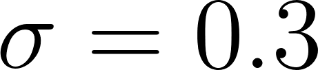 , and the only question is which arm to pull next. The
scoreboard is regret, the reward given up compared with always pulling
the best arm:
, and the only question is which arm to pull next. The
scoreboard is regret, the reward given up compared with always pulling
the best arm:
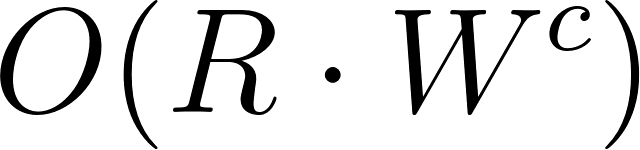
bandits.rkt uses the standard ten-armed Bernoulli test bed from Sutton
and Barto, whose arm means range from 0.10 to 0.85. Each strategy is a
bandit-agent struct holding two closures: choose returns an arm, and
update! folds in the reward. One benchmark loop then runs any strategy,
and a fresh agent per run keeps the statistics clean.
The strategies, and the idea behind each:
- greedy — always take the best estimate so far. It is the fastest learner if the first pulls happen to be lucky, and hopeless if they are not.
- epsilon-greedy — explore a uniformly random arm with probability
 . The estimate can be a plain sample average (right for a
stationary problem) or a constant step size
. The estimate can be a plain sample average (right for a
stationary problem) or a constant step size  that forgets old
rewards (right when the means move).
that forgets old
rewards (right when the means move).
- optimistic initialization — start every arm at +5. Greedy exploitation then is exploration, until each arm has been tried once.
- UCB1 — pull the arm maximizing
Q(a) + c\sqrt{\log t / N(a)}$: a bonus that shrinks as an arm is used, so under-tried arms stay attractive. Total regret grows logarithmically instead of linearly. - Thompson sampling — keep a
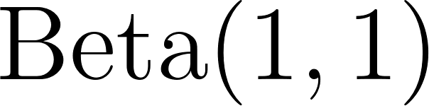 posterior per arm,
draw one sample per arm, pull the largest. Exploration is automatic: an
arm with little evidence has a wide posterior. (A Beta sample is built
from two integer-shape Gamma samples, and a Gamma sample is a sum of
exponentials — see
posterior per arm,
draw one sample per arm, pull the largest. Exploration is automatic: an
arm with little evidence has a wide posterior. (A Beta sample is built
from two integer-shape Gamma samples, and a Gamma sample is a sum of
exponentials — see random-gamma-int.) - softmax — sample arm
awith probability proportional toe^{Q(a)/\tau}$.
Two hundred runs of a thousand pulls each give the following table, where every number is reproducible from the fixed seed:
1 strategy               regret@100   regret@500  regret@1000 % best arm
2 greedy                 74.98        375.03      750.62      0.000
3 epsilon-greedy 0.1     34.26        66.10       89.47       0.740
4 epsilon-greedy 0.01    68.04        226.83      314.27      0.284
5 optimistic init 5      11.52        32.49       57.97       0.710
6 ucb1 c=1               26.05        73.00       98.44       0.684
7 thompson sampling      19.17        32.98       37.08       0.877
8 softmax tau=0.1        20.33        67.06       104.27      0.545
Three things are worth reading off this table.
First, greedy never recovers. Its regret curve is a straight line: it
locks onto an arm that paid early and stops learning, so it never finds the
0.85 arm. -greedy at 0.01 is almost as bad, because its rare
exploration is not targeted.
Second, optimistic initialization explores well but only once. Its curve is nearly flat after the first hundred pulls — the initial optimism is gone and nothing keeps re-testing arms.
Third, uncertainty-aware methods win. Thompson sampling reaches 0.877 of pulls on the best arm with less total regret than any other strategy, and UCB1 is close behind while actively balancing arms. Their regret grows sublinearly because they keep spending pull budget where the evidence is thin.
The second half of the demo repeats the comparison on a drifting bandit:
after every pull each mean takes a small Gaussian step. Now the best arm
changes over time, total regret is a moving target, and the fair question
is how much reward the agent earns in the last two hundred pulls. The
sample-average -greedy learner cannot forget its early evidence
and tracks poorly; the constant- version, which weighs recent
rewards more heavily, does better. This is the classic argument for
exponential recency weighting in Chapter 2 of Reinforcement Learning: An
Introduction.
Part 2: Tabular temporal-difference control
Bandits have no state, so nothing that is learned in one situation has to
transfer to another. Add states and the problem becomes a Markov decision
process: the agent observes a state  , picks an action
  , receives a
reward
, receives a
reward  and lands in
 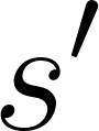 . The quality of a decision now depends on
what happens afterwards, which is what the discount factor
. The quality of a decision now depends on
what happens afterwards, which is what the discount factor
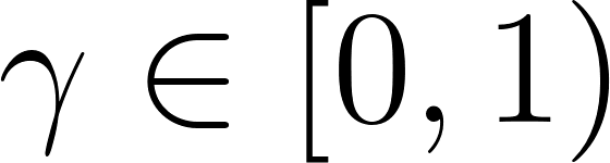 and the action-value function
 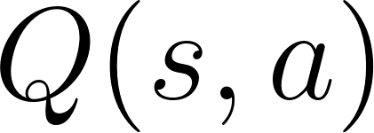 capture.
The GridWorld test bed
environments.rkt defines the maze used throughout:
1 S . . . .
2 . # . # .
3 . . . # .
4 # # X . .
5 . . . . G
S is the start, G the goal (reward +1 and the episode ends), X a pit
(reward -1 and the episode ends), and # walls, which block movement. Any
other step costs 0.01, so the agent prefers short routes. With
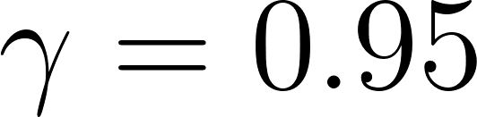 the optimal discounted return from
 S is 0.6380,
reached by walking right along the top edge and then down the right edge:
1 → → → → ↓
2 ↑ # ↑ # ↓
3 ↑ → ↑ # ↓
4 # # X → ↓
5 → → → → G
Two features of the implementation matter. First, gridworld-transitions
exposes the model as a list of (probability, next-state, reward, terminal?) tuples, while gridworld-step samples from exactly the same
distribution. The TD methods only ever call the sampler, but value
iteration uses the model, so the learned tables can be compared with the
exact optimum. Second, states are integers 0…24 and the Q table is a
vector of 25 rows of four numbers.
Four methods, one episode loop
All four methods start from the same update shape,

and differ only in  :
:
| Method | Target y$ |
Policy |
|---|---|---|
| Q-learning |
r + \gamma \max_{a'} Q(s',a')$ |
off-policy |
| SARSA |
r + \gamma Q(s',a')$, with a'$ the action epsilon-greedy will take |
on-policy |
| Expected SARSA |
r + \gamma \sum_{a'} \pi(a' \mid s') Q(s',a')$ |
on-policy |
| Double Q-learning | update Q_1$, bootstrap \arg\max$ from Q_1$ evaluated in Q_2$ (and vice versa on a coin flip) |
off-policy |
The distinction between on-policy and off-policy is not academic. SARSA
asks “how good is the policy I am actually following, exploration and
all?”, while Q-learning asks “how good is the greedy policy?”. The epsilon
exploration near the pit therefore makes SARSA’s values lower than  there, and it can even prefer to bump into a wall where nothing bad can
happen. Q-learning never pays that price because it bootstraps from a
maximum rather than from its own next action.
there, and it can even prefer to bump into a wall where nothing bad can
happen. Q-learning never pays that price because it bootstraps from a
maximum rather than from its own next action.
Training each method for 800 episodes with 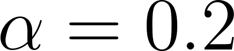 and
annealed from 1.00 to 0.05 over the first 400 episodes gives:
and
annealed from 1.00 to 0.05 over the first 400 episodes gives:
1 method           return     success   steps    mean|dQ|
2 q-learning       0.6380     1.000     8.00     0.0600
3 sarsa            0.6380     1.000     8.00     n/a (on-policy)
4 expected-sarsa   0.6380     1.000     8.00     n/a (on-policy)
5 double-q         0.6380     1.000     8.00     0.1291
6
7 Value iteration reference: V(start) = 0.6380 after 8 sweeps
All four find the optimal route. The mean|dQ| column averages the
difference from the exact over state-action pairs that were visited
at least five times. Q-learning is closest (0.06) because its target is
; SARSA and expected SARSA are deliberately marked n/a because
they converge to the value of the epsilon-greedy behaviour policy, not to
. Comparing them with would be comparing two different
questions.
Check your answers with dynamic programming
Value iteration sweeps Bellman’s optimality equation

until the largest change falls below 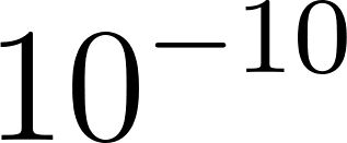 ; on this maze it needs
eight sweeps, one per step of the horizon, and produces the exact
; on this maze it needs
eight sweeps, one per step of the horizon, and produces the exact 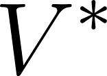 and . Having a model-based answer is not cheating — it is how the
sampled methods in the rest of the chapter are verified, and how the
and . Having a model-based answer is not cheating — it is how the
sampled methods in the rest of the chapter are verified, and how the
 and reward choices were checked in the first place.
Part 3: Policy gradient methods
Q-learning learns values and reads a policy off them. Policy gradient
methods parameterize the policy itself and follow the gradient of expected
return. For a softmax policy over action scores  ,
,
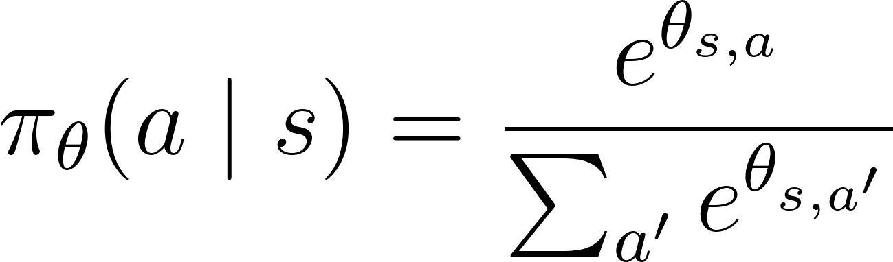
the score-function estimator says: run an episode with the current policy, and for each step push up the log-probability of the action that was taken, weighted by the return that followed,

The expectation of this update is the policy gradient. In code the whole
thing is three lines, because the gradient of a softmax log-probability
with respect to the score of action is just 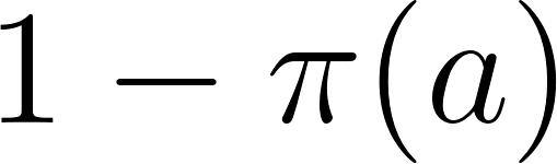 when
was taken and
when
was taken and 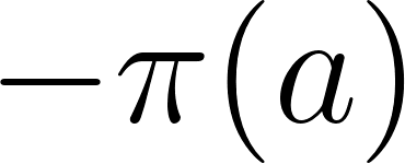 otherwise.
Three refinements make it work in practice, and policy_gradient.rkt
turns each on and off so the difference is visible:
- Subtract a baseline.
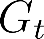 can be several hundred in CartPole, so
the raw updates have enormous variance. Subtracting any quantity that
does not depend on the action leaves the gradient unbiased and shrinks
the noise.
can be several hundred in CartPole, so
the raw updates have enormous variance. Subtracting any quantity that
does not depend on the action leaves the gradient unbiased and shrinks
the noise.
- Discount and normalize the returns. One long lucky episode should not dominate the update, so returns-to-go are discounted and (on CartPole) standardized to zero mean and unit variance.
- Add an entropy bonus.
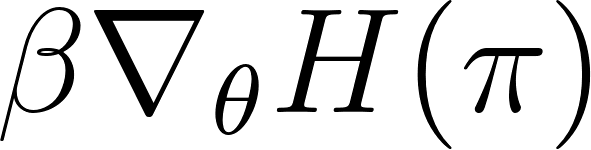 keeps the
policy from collapsing onto one action before it has learned anything.
keeps the
policy from collapsing onto one action before it has learned anything.
A baseline must know about states
The GridWorld comparison is the most instructive result in this chapter:
1 variant                  sampled ret  greedy ret   success   steps
2 raw-returns              0.5140       0.6380       1.000     8.00
3 mean-baseline            -0.2421      -0.1988      0.000     100.00
4 learned-value-baseline   0.4409       0.6380       1.000     8.00
5 value-baseline-entropy   0.3057       0.6380       1.000     8.00
Subtracting the mean return of the episode makes the learner worse,
not better. The reason is subtle and worth stating carefully. With a
terminal reward, every return-to-go in a failed episode is nearly the
same number (-1 for the pit). Subtracting the episode mean leaves an
advantage near zero, so the update does not change the probabilities of
the actions on that trajectory at all — the learner never finds out that
the states along the way were bad. It only learns from successful
episodes, and never learns to avoid the pit. A learned 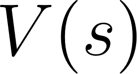 is
state-dependent: entering a pit makes
is
state-dependent: entering a pit makes 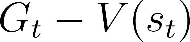 strongly negative,
the policy backs away, and the maze is solved. The lesson generalizes:
baselines should explain the state, not just the episode.
strongly negative,
the policy backs away, and the maze is solved. The lesson generalizes:
baselines should explain the state, not just the episode.
From a table to a function
GridWorld has 25 states, so a 25x4 score table is fine. CartPole has four continuous state variables — position, velocity, pole angle, angular velocity — so there is no table to write. The fix is to compute the scores from features:

Feature scaling is not optional here. The raw variables have very
different ranges (the angle stays within 0.21 rad while velocities reach
several units), so cartpole-observe divides each by a rough scale and
appends a bias term. With that, REINFORCE plus Adam — note the gradient
sign, since Adam descends and this is an ascent problem — learns to
balance the pole:
1 Mean episode length per 100-episode block (training):
2   35.9  220.7  375.4  441.0  460.6  450.9
3
4 Greedy evaluation over 20 episodes: mean 500.0 steps, best 500, 20/20 reached 500.
A random policy survives about 22 steps and the hard limit is 500, so the linear policy is balancing the pole indefinitely. A linear policy is enough for CartPole because the task really is almost linear: push in the direction the pole is falling, harder when it is falling faster.
Part 4: Deep Q-Networks
The last example replaces the Q table with a neural network so that
Q-learning can handle continuous states. neural_net.rkt provides the
smallest thing that works: fully connected layers with ReLU or tanh
activations, backpropagation, and Adam. Weights and gradients are flat
flvectors laid out row-major, and a finite-difference test in tests.rkt
checks the analytic gradients before any of it is used for learning.
Naively training a network on the Bellman target does not work: samples
arrive in a correlated stream from a single trajectory, the target moves
every time the network changes, and a single large TD error can destroy
the weights. DQN’s three fixes are all present in dqn.rkt:
- Replay buffer. The last 5000 transitions are stored in a ring buffer and minibatches of 32 are drawn uniformly at random, which breaks the correlation between consecutive updates.
- Target network. A frozen copy of the network, recopied every 250 steps, supplies the bootstrap value
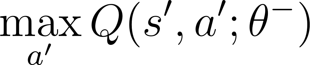 .
The target then changes slowly instead of chasing the prediction.
.
The target then changes slowly instead of chasing the prediction.
- Huber (clipped) TD error. The loss is quadratic for small errors and linear beyond
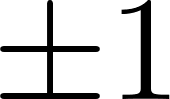 , so one surprising transition cannot produce
a huge gradient.
, so one surprising transition cannot produce
a huge gradient.
The GridWorld demo uses one-hot state vectors, which makes the network a differentiable Q table and allows a direct numerical comparison:
1 Network 25 -> 48 -> 48 -> 4 (ReLU, linear output)
2 Training return per 50-episode block:  -0.64  0.74  0.83  0.85  0.91
3
4 Greedy evaluation over 200 episodes: mean return 0.6380, success 1.000, mean 8.00 steps.
5 Value iteration optimum:                                    0.6380, success 1.000, 8.00 steps.
6
7 mean |Q - Q*| over all 100 state-action pairs:
8   DQN network        0.1718
9   tabular Q-learning 0.0600
Both reach the optimal return of 0.6380. The network’s values are a little noisier than the table’s, which is the price of gradient-based function approximation, but the greedy route is the same eight moves.
Only the input features change between GridWorld and CartPole:
racket dqn.rkt --cartpole feeds the four scaled state variables to a
4-64-64-2 network with the same replay buffer, target network and Huber
loss. CartPole is much harder for DQN than for the linear policy gradient
above, and the comparison is a lesson in sample efficiency. After 300
episodes the greedy policy survives 106.8 steps on average (best 112),
where a random policy survives about 22 — the network has discovered the
balancing rule but has not mastered it — while the linear policy gradient
balances for the full 500 steps in 600 episodes. The linear policy starts
with the right inductive bias: its inputs are position, velocity, angle
and angular velocity, exactly the quantities a balancing control law
needs, and the network has to learn that mapping from a scalar reward
signal. The demo is scored on its greedy policy rather than on training
episode lengths, because the epsilon schedule is still exploring while
training.
Where the sharp edges are
RL code fails quietly: it runs, produces numbers, and the numbers are
wrong. Four bugs found while writing this chapter are documented in
source-code/ReinforcementLearning/PROBLEMS.md, and each is worth knowing
about:
- Double Q-learning must flip its coin before the terminal check, otherwise terminal data all lands in one table and the other table starves.
- Thompson sampling must sum exponentials rather than multiply uniforms; after a few hundred pulls the product underflows and every arm gets the same saturated sample.
- Adam is a descent optimizer; a REINFORCE gradient must be negated before it is applied, or the policy learns to minimize the return.
- Seed the PRNG before building the network, or the weights differ from process to process and the demo is not reproducible.
Exercises
- Add EXP3 to
bandits.rkt. It maintains exponential weights over arms and works even when the rewards are chosen adversarially rather than sampled from fixed means. Compare its regret on the drifting bandit with Thompson sampling. - Track non-stationarity properly. Give the bandit driver a “reward in the last 200 pulls” metric for every strategy and find the drift rate at which sample-average epsilon-greedy finally loses to the constant-alpha version.
- Implement n-step Q-learning. Replace the one-step target in
q_learning.rktwith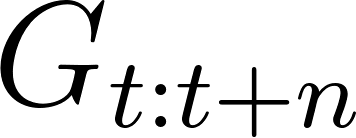 and see how the maze’s learning
curve changes for
and see how the maze’s learning
curve changes for  (the maze’s horizon is eight
moves).
(the maze’s horizon is eight
moves).
- Add eligibility traces. SARSA(
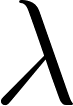 ) with replacing traces is
only a few lines on top of the tabular table; measure how much faster
it reaches the optimal policy than one-step SARSA.
) with replacing traces is
only a few lines on top of the tabular table; measure how much faster
it reaches the optimal policy than one-step SARSA.
- Double DQN. In
dqn.rkt, choose the maximizing action with the online network and evaluate it with the target network, and count how often the plain DQN’s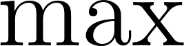 overestimates the true .
- Soft target updates. Replace the hard target-network copy with Polyak averaging,
 ,
and tune
,
and tune  on CartPole.
- Prioritized replay. Sample transitions in proportion to their TD error instead of uniformly. The replay buffer in
dqn.rktis a ring buffer, so this is a real change to the data structure, not just the sampling distribution. - Advantage actor-critic. Reuse
neural_net.rktto learn
with the network, subtract it from the returns to get advantages, and
compare with the tabular baseline in policy_gradient.rkt. - Change the world.
make-gridworldtakes walls, pits, rewards, start and goal, and even a slip probability, so the same code can test a stochastic maze. Which methods survive when the agent slips 30% of the time?