Deep Learning in Racket with Malt: From XOR to a Two-Tower Recommendation System

A single linear model can only draw straight boundaries. Feed it the four input/output pairs of the XOR function, like: (0,0)→0, (0,1)→1, (1,0)→1, (1,1)→0 and it fails no matter how long you train it, because no straight line separates the 1s from the 0s. This was the famous critique that stalled neural network research in 1969, and it has a famous resolution: stack layers with a non-linear function (here, the rectifier , or ReLU) between them. One hidden layer is enough to bend the decision boundary around the XOR pattern.

That is the thread running through this chapter’s three examples:

1. XOR: the smallest problem that requires a hidden layer.
2. Circle classification: a two-hidden-layer network learning a curved boundary from synthetic data we generate ourselves.
3. A two-tower recommender: a jointly learned model that takes two kinds of input (customer features and product features), learns an embedding for each, and predicts a rating. Along the way we hit, diagnose, and fix a real bug: and the debugging trail is as instructive as the model itself.

Malt is the deep learning library built for The Little Learner (the third book in the Little Schemer series). Three ideas suffice for everything in this chapter:

• Tensors. Nested arrays of numbers: a scalar is rank 0, a vector rank 1, a matrix rank 2. (tensor 1.0 2.0) builds one; (tref t i) indexes it.
• Layers as functions of two arguments. A layer such as relu is a function that takes the input tensor and returns a function of theta (the parameter list). A network is then just function composition, and block/stack-blocks package layers together with their parameter shapes:

  1 (block relu (list (list 8 2) (list 8)))  ; weights (8×2) + bias (8)
  

• Gradient descent. l2-loss turns a network into a loss function, sampling-obj makes it stochastic (mini-batches), and naked-gradient-descent optimizes it using automatic differentiation (∇). Hyperparameters (e.g., revs (iterations), alpha (learning rate), batch-size) are set with with-hypers.

So that no listing below sends you reaching for a browser, here is the complete vocabulary of the chapter. Functions are explained at first use as well; treat this as the reference you can flip back to.

Building and inspecting tensors

• (tensor ...): constructs a tensor from numbers or other tensors. (tensor 1.0 2.0) is a rank-1 vector; (tensor (tensor 1 2) (tensor 3 4)) is a 2×2 matrix. Tensors must be rectangular: every row the same length.
• (list->tensor lst): converts a (possibly nested) list into a tensor. This is the workhorse for programmatic data generation: build a list with for/list, then convert.
• (tref t i): tensor ref: element i of t. (tref (tensor 7 8 9) 1) is 8. Works at any rank: on a matrix it returns a row.
• (tlen t): tensor length: the size of the outermost dimension.
• (shape t): the dimensions as a list, e.g. (400 7) for a data tensor of 400 samples of 7 features.
• (concat u v): concatenates two rank-1 tensors end to end. Differentiable, so gradients flow through it.
• (dot-product-2-1 W t): matrix × vector: W is rank 2, t rank 1, and each row of W is dotted with t. This is the “multiply by the weight matrix” half of every neural network layer.
• (flatten t): collapses a tensor to rank 1.

Layers and networks

• linear :the affine layer. ((linear t) theta) computes W·t + b, where theta is the list (weights bias). (You will never write the multiplication yourself.)
• rectify: the ReLU activation, , applied elementwise.
• relu: linear followed by rectify: the standard fully-connected layer used in all three examples.
• (block fn shape-list): bundles a layer function with the shapes of its parameters. (block relu (list (list 8 2) (list 8))) means: a relu layer whose theta is an 8×2 weight matrix plus a bias vector of 8.
• (stack-blocks (list b1 b2 ...)): composes blocks left to right into a network, wiring the output of each block into the next and concatenating their parameter lists.
• (block-fn network): extracts the composed function from a stacked network: something you can call as ((fn input) theta).
• (block-ls network): extracts the list of parameter shapes from a network. You need it to create correctly-shaped initial parameters; for the XOR network it returns ((8 2) (8) (1 8) (1)), e.g., weight matrix and bias for the hidden layer, then weight matrix and bias for the output layer.

Parameters, training, and prediction

• (init-theta shapes): creates fresh parameters with the given shapes: random small weights, zero biases. This is the starting point that gradient descent improves.
• (l2-loss fn): given a network function, returns a loss function of the training data and theta: the average squared difference between the network’s predictions and the targets. “L2” refers to the L2 (Euclidean) norm, the straight-line distance between two vectors. Concretely, for a batch of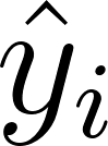 samples, where is the network’s prediction and the true target, the L2 loss is the mean of squared errors:

Squaring does two jobs at once: it makes every error positive (over- and under-predictions can’t cancel), and it penalizes large errors much more than small ones: a prediction off by 1.0 costs 100× more than one off by 0.1, so gradient descent is pushed hardest exactly where the model is most wrong. Just as important for us, the square function has a simple, smooth derivative everywhere, which is what makes the loss a good target for automatic differentiation. (Malt also offers cross-entropy-loss for probability outputs and kl-loss for matching distributions; L2 is the natural choice here because our targets are plain numbers, not probabilities.)

The value returned by l2-loss is not a number but a function waiting for data: ((l2-loss fn) xs ys) is itself a function of theta, and that is the object gradient descent knows how to minimize.

• (sampling-obj loss xs ys): wraps the loss so each evaluation uses a random mini-batch drawn from xs/ys (stochastic gradient descent). The batch size comes from the batch-size hyperparameter.
• (naked-gradient-descent objective theta0): plain SGD. Repeatedly compute the gradient of objective with respect to theta and steps downhill. It returns the trained theta. (“Naked” distinguishes it from the momentum/velocity/RMSProp/Adam variants malt also provides.)
• (with-hypers ((revs n) (alpha a) (batch-size b)) body): runs body with hyperparameters in scope: revs is the number of gradient steps, alpha the learning rate, batch-size the mini-batch size.
• (model fn theta): freezes trained parameters into a bare prediction function: ((model fn theta) input) is the network applied to one input, no theta argument needed.
• (∇ f theta) (also gradient-of): automatic differentiation. The gradient of scalar function f with respect to theta. Used internally by gradient descent; used by us directly when debugging.
• (dual? x) / (ρ x): malt implements AD by wrapping numbers in duals that carry a derivative. Trained thetas and model outputs can contain duals; dual? detects them and ρ (“rho”) extracts the plain numeric value. The examples define (define (realize x) (if (dual? x) (ρ x) x)) for this.

List helpers malt provides (used for walking the parameter list): ref/tref-style indexing with (ref lst i), (refr lst i) (“ref rest”: drop the first i elements), and len. In the recommender, (refr theta 2) means “theta starting at the product tower’s parameters”.

Install malt once with:

The network is 2→8→1: eight ReLU units in one hidden layer, one output unit. The training set is the entire function: four input vectors and their targets:

Read the network definition as a data-flow diagram: stack-blocks wires two relu blocks in series, and block-ls recovers the parameter shapes from that definition; for this network, ((8 2) (8) (1 8) (1)). That shape list is exactly what init-theta needs to manufacture a random starting theta, so the network architecture is written down once and everything else is derived from it. Training is then a single naked-gradient-descent call over 4000 revisions with the whole dataset (batch size 4) as each mini-batch: l2-loss builds the loss function from the network, sampling-obj adapts it to mini-batch sampling, and with-hypers supplies the knobs. The complete file, xor.rkt:

The outputs are 0.000… and 0.999…: the network has learned XOR exactly, to floating-point precision. Two practical notes. First, ReLU networks can collapse at initialization (all units dead, every prediction identical); if you see that, change the random seed or lower the learning rate. Second, malt prints some startup noise ("settings=" hash lines); filter it with 2>/dev/null if it bothers you.

XOR’s boundary problem is tiny. A more realistic test: scatter 300 random points in the square [-1,1]×[-1,1] and label each 1 if it lies inside a circle of radius 0.6, 0 otherwise. A representative sample of the data as generated (two coordinates in, one label out):

The network is 2→8→8→1, with two hidden layers. Depth matters here: the first layer can carve the plane into half-planes; the second can combine those into polygonal regions that approximate the circle. The data generator and the rest of two_hidden_layers.rkt:

The label generator deserves a close look: for each of the 300 samples, tref twice digs out the coordinates: (tref circle-xs i) is the i-th sample (a 2-vector), and a second tref picks the x or y coordinate; then the label is 1.0 exactly when 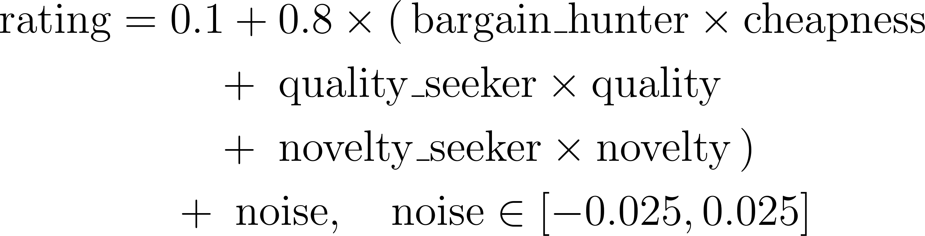. The self-check at the bottom applies the trained circle-model to every training point and counts how often the thresholded prediction (> pred 0.5) matches the label; that for/sum pattern (model in, count out) is the minimal viable test harness for every network in this chapter.

Two idioms worth noting. The data is built with plain Racket for/list loops wrapped in list->tensor, the most reliable way to construct tensors programmatically in malt. And we call (random-seed 1) again right before init-theta, because data generation consumed the random stream; re-seeding makes the initial weights reproducible.

299 of 300 training points are classified correctly (predictions are thresholded at 0.5). The sample predictions show the learned geometry: the origin (0,0) and the inner point (0.3, 0.2), both inside the circle, score above 1, while the far corner (0.9, 0.9) and the point (-0.8, 0.5) (radius ≈ 0.94, outside) score 0. ReLU networks are free to overshoot the nominal [0,1] range; nothing in the architecture clamps the output, and with l2 loss it doesn’t need to.

Real recommendation systems rarely see one flat feature vector. They see different kinds of things (a customer and a product) and must model the interaction between them. The standard trick is to give each input type its own sub-network (“tower”) that compresses raw features into a learned embedding, then combine the embeddings to produce a score. Both towers are trained jointly: the same gradient signal shapes what the model learns about customers and about products.

Our synthetic world: customers are described by 3 numbers in [0,1): how much of a bargain hunter, quality seeker, and novelty seeker they are. Products get 4 numbers: cheapness (inverse price), quality, popularity, and novelty. The hidden ground truth is a taste match:

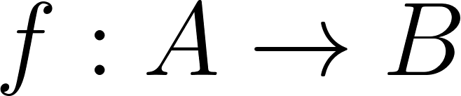
Note the multiplications: a rating depends on products of customer and product features. Popularity is deliberately unused, a decoy feature the model should learn to ignore. A sample of the generated data (400 samples, inputs concatenated into one 7-element vector, customer first):

The input is one 7-element tensor. Malt has no slice operation and tensors must be rectangular (so we can’t pass a ragged pair of vectors), so we slice with constant 0/1 selection matrices: multiplying the input by a 3×7 identity-prefix matrix extracts the customer features, and a 4×7 identity-suffix matrix extracts the product features. A dot-product with a constant matrix is differentiable, so gradients flow through the slices. Each half then goes through its own linear+rectify tower (producing a 4-element embedding), the embeddings are concatenated, and a final linear layer emits the rating.

One malt subtlety appears in the code below: trained parameters and model outputs can contain duals (malt’s automatic-differentiation wrappers), so we unwrap them with ρ before doing plain arithmetic, and we import a few racket/base operators under aliases (r+, r-, …) for scalar bookkeeping, since malt redefines + - * / as binary differentiable tensor operations.

The complete joint_recommendation.rkt:

Because this network is a custom composition rather than a stack-blocks chain, we manage theta explicitly: rec-theta-shapes declares the six parameter tensors (two per layer), and refr in the block function walks the parameter list: theta for the customer tower, (refr theta 2) for the product tower, (refr theta 4) for the output layer.

Walk through rec-block-fn one expression at a time. The customer half of the input is (dot-product-2-1 select-customer t), a 3-element vector pulled out of the 7-element input. ((linear ...) theta) applies the customer tower’s affine transform (consuming theta[0], the 4×3 weights, and theta[1], the bias), and rectify makes it non-linear: the result is cust-emb, a 4-element learned embedding of the customer. The product tower is identical except it reads (refr theta 2), the parameter list with its first two elements skipped, so linear there sees theta[2] and theta[3] as its weights and bias. (concat cust-emb prod-emb) glues the two 4-element embeddings into one 8-element vector, and the final linear over (refr theta 4) reduces that to a single number: the predicted rating. Every operation in the chain is differentiable, so naked-gradient-descent shapes all six parameter tensors from the same loss signal. The two towers and the head learn jointly, each adapting to what the others produce.

The scoring of a new customer at the end shows the intended use of a recommender: the customer vector is fixed, and we concatenate it with each candidate product in turn ((concat new-customer p) rebuilds the 7-element input layout the towers expect), reading off a predicted rating per product.

The mean absolute error of 0.09 on targets ranging from ~0.16 to ~1.61 means the model captures the taste-match structure well. For the new customer (a bargain hunter (0.9) and quality seeker (0.8) who doesn’t care about novelty (0.1)) the model scores the cheap, high-quality product highest and the mid-priced, low-quality novelty item lowest, exactly as the ground-truth formula dictates. It slightly over-values the expensive popular product (the ground truth says 0.82 vs. the predicted 1.02): a concat-then-linear head can only approximate multiplicative interactions, so some residual distortion is expected. If we needed a tighter fit, the principled move would be to score with a dot-product of the two embeddings, the classic matrix-factorization head, which matches the bilinear structure of the data exactly.

The first version of the recommender trained to MAE 0.25 and predicted the same constant (~0.72) for every product; essentially the mean rating. The debugging trail is worth following because each step is a general technique:

1. Check the data first. sanity_check.rkt recomputed targets by hand with base arithmetic and verified shapes, values, and distribution, all correct. (The synthetic data generator is included in this directory for exactly this purpose.)
2. Check the gradients. Evaluating (∇ ...) on a single sample showed every weight gradient exactly 0.0 while bias gradients were fine, identically across all inputs. Identical zeros are never dead ReLUs; they mean structure, not luck.
3. Bisect the composition. Each primitive (dot-product-2-1, concat, linear) passed gradients in isolation, and the two-tower architecture worked with hand-written literal matrices, which pointed at the matrix construction.

The culprit was one line in selection-matrix:

Malt redefines + as a differentiable operator whose results are never eq? to plain integers, so the condition was silently always false and the “selection matrices” were all zeros. The towers received zero vectors; with malt’s zero-initialized biases, the embeddings rectified to 0; every weight gradient vanished; only the final bias could move, and a lone bias can only learn the mean. The fix uses base operators for index arithmetic: (equal? j (r+ i offset)). MAE dropped from 0.25 to 0.09 with no other change.

The general lesson: when a model collapses to predicting the mean, suspect the gradient path before the hyperparameters. And in malt, remember that + - * / abs min max sub1 are no longer the racket/base versions.

• malt shadows + - * / abs min max sub1 with binary, differentiable tensor ops. (+ a b c) fails deep in D-extend.rkt; sub1 rejects inexact numbers. Alias base ops (r+ etc.) for scalar bookkeeping.
• Never compare the result of malt arithmetic with eq?.
• Model outputs and trained parameters may be duals. Unwrap with (if (dual? x) (ρ x) x) before plain math.
• Tensors must be rectangular; use list->tensor + for/list to build them, and constant selection matrices to slice them.
• Re-seed right before init-theta for reproducible runs; if training collapses to a constant, try another seed or a smaller alpha before redesigning the network.