Category-Theory Deep Learning in Racket
Deep learning is usually taught as a pile of engineering tricks: activation functions, backprop, dropout, weight decay. This chapter takes the opposite route. We build a small but complete deep-learning framework in Racket whose design is dictated by category theory — the mathematics of structure and composition. Every component you would normally bolt on ad hoc (gradient descent, dropout, uncertainty estimates, invariance, ensembling) turns out to be a named categorical construction with precise laws.
The framework is a working implementation of the survey by Jia, Peng, Yang & Chen (2025), “Category-Theoretical and Topos-Theoretical Frameworks in Machine Learning”, Axioms 14(3):204 (https://doi.org/10.3390/axioms14030204). By the end of the chapter you will have ~285 lines of Racket that train an XOR network, implement dropout as a lens, estimate predictive uncertainty by Monte Carlo, run k-means as a colimit computation, classify via a topos’ subobject classifier, glue ensemble predictions like sheaf sections, and distill knowledge through a natural transformation.
Why category theory for machine learning
A category is a collection of objects with morphisms (arrows) between them, where morphisms compose associatively and every object has an identity morphism. That sounds abstract, but it is exactly the structure machine learning already has:
- Networks are built by composing layers.
- Loss functions compose with models.
- Ensembles combine predictors.
- Architectures are distinguished by which transformations they commute with.
Category theory’s payoff is that when you recognize your construction as a known pattern (a lens, a Markov category, a colimit, a sheaf), you get its laws, its composition rules, and its proofs for free — rather than discovering each one by trial and error. The survey organizes categorical ML into five perspectives, and this chapter implements all five:
| Perspective | Categorical idea | What we build |
|---|---|---|
| I. Gradients | Para category, lenses | Compositional backprop, SGD as an endomorphism |
| II. Probability | Markov categories | Dropout as a stochastic lens, Bayesian uncertainty |
| III. Symmetry | Equivariance, colimits | Permutation-invariant pooling, k-means |
| IV. Truth | Topos, subobject classifier, sheaves | Binary decisions, ensemble gluing |
| V. Reuse | Natural transformations | Knowledge distillation |
The mathematics of the five perspectives
I. The Para category and lenses
In the Para construction, a neural-network layer is a parametric morphism
 : it consumes an input from
  and produces an output in
  ,
but it does so using parameters living in a separate space
,
but it does so using parameters living in a separate space  . So a layer is
really a map
. So a layer is
really a map

To train such a layer we need to know how a small change in its output propagates back to its parameters and its input. That bidirectional pair — a forward map plus a pullback — is a lens. The forward pass of a layer is the “get” direction; the backward pass is the “put” direction:

The crucial theorem is that lenses compose. Chaining layers composes their
forward passes, and backpropagation is nothing but composing the pullbacks in
the reverse order — a covariant functor on the gradient category. The SGD
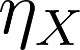
update 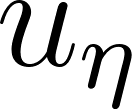 is then simply an
endomorphism
is then simply an
endomorphism  on the model object.
II. Markov categories
A Markov category is the right setting for stochastic computation. Its morphisms are stochastic kernels: given an input, they return a probability distribution over outputs. From a programming point of view, a stochastic morphism is just a function that samples.
Two ML staples are stochastic morphisms in disguise. Dropout multiplies
activations by a Bernoulli mask sampled at train time — a stochastic lens
whose forward pass samples the mask and whose backward pass reuses the same
mask (the closed-optic requirement). Bayesian layers treat weights as
random variables, sampling 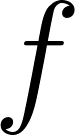 at every
forward pass; the spread of many forward passes measures epistemic
uncertainty.
at every
forward pass; the spread of many forward passes measures epistemic
uncertainty.
III. Invariance, equivariance, and colimits
A layer  is equivariant under a group
  when
when 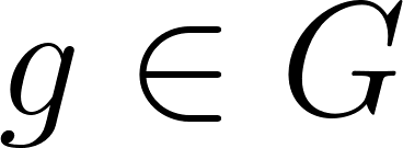 for every
  : the symmetry of the input is preserved by the layer.
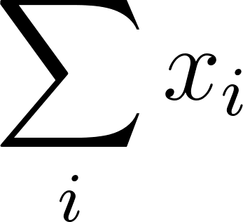
Invariant maps go further and forget the symmetry entirely. The sum
: the symmetry of the input is preserved by the layer.
Invariant maps go further and forget the symmetry entirely. The sum
 is invariant to any permutation of its inputs — it is the
colimit (coproduct) over the set diagram, and it is the heart of
set-based architectures like DeepSets. In the same spirit, k-means clustering
is a colimit computation: each cluster centroid is the colimit (average) of
the points in its cluster, and point-to-centroid assignment is the universal
morphism.
is invariant to any permutation of its inputs — it is the
colimit (coproduct) over the set diagram, and it is the heart of
set-based architectures like DeepSets. In the same spirit, k-means clustering
is a colimit computation: each cluster centroid is the colimit (average) of
the points in its cluster, and point-to-centroid assignment is the universal
morphism.
IV. Toposes: subobject classifiers and sheaves
A topos is a category rich enough to do logic inside it. Its key ingredient is
the subobject classifier  : a special object with a “true” arrow
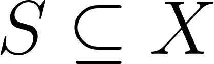 such that every subset
  is picked out by a
unique characteristic morphism
is picked out by a
unique characteristic morphism 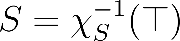 with
with
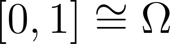 . In machine learning, the sigmoid output of a binary
classifier is such a characteristic morphism: it maps inputs into
. In machine learning, the sigmoid output of a binary
classifier is such a characteristic morphism: it maps inputs into
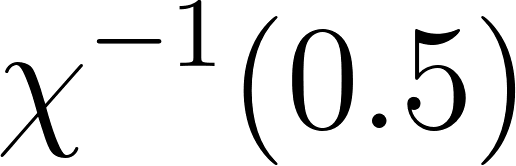 , and the decision boundary is
 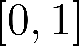 .
.
A sheaf packages local data that must agree on overlaps. If you think of
each model in an ensemble as an expert covering its own local context, then
combining their predictions requires the sheaf condition: on shared context,
experts must agree. Consistent sections glue into a global prediction;
inconsistent ones reveal disagreement. Finally, carries a Heyting
algebra (intuitionistic logic); on  it collapses to
 ,
,  ,
,  .
.
V. Natural transformations
Given two functors 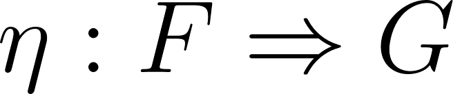 and , a natural transformation
  is a family of morphisms
  that commutes with every
arrow — a structure-preserving way to convert one kind of computation into
another. Knowledge distillation is exactly this: a small “student” model
learns to reproduce the hidden representations of a large “teacher”. The
adapter between teacher and student representations is
that commutes with every
arrow — a structure-preserving way to convert one kind of computation into
another. Knowledge distillation is exactly this: a small “student” model
learns to reproduce the hidden representations of a large “teacher”. The
adapter between teacher and student representations is  .
.
The data
Before we look at any parsing or training code, here is the data it processes.
The framework stores each example as a pair  .
.
XOR, the canonical non-linearly-separable problem. Four points in the unit square, where the target is 1 exactly when the two inputs differ:
1 ((0.0 0.0) 0.0)
2 ((0.0 1.0) 1.0)
3 ((1.0 0.0) 1.0)
4 ((1.0 1.0) 0.0)
Dropout demo. One five-vector that we will push through the dropout lens, plus the unit gradient we backpropagate through it:
1 (1.0 2.0 3.0 4.0 5.0)     ; activations
2 (1.0 1.0 1.0 1.0 1.0)     ; upstream gradient
Bayesian demo. A three-dimensional input for the single-output Bayesian layer, which we will query 200 times:
1 (1.0 0.5 -0.5)
Cluster data. Nine points in the plane arranged in three obvious clusters: three near (1,1), three near (5,5), and three near (1,5):
1 (1.0 1.0) (1.2 0.8) (0.9 1.1)
2 (5.0 5.0) (5.1 4.9) (4.8 5.2)
3 (1.0 5.0) (0.9 4.8) (1.1 5.1)
Sheaf sections. Three “expert” predictions on overlapping contexts, two of which agree within tolerance and one of which does not:
1 section A: prediction 0.72
2 section B: prediction 0.68
3 section C: prediction 0.91
All randomness is seeded (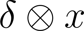 ) so every run reproduces the exact
outputs shown later in this chapter.
) so every run reproduces the exact
outputs shown later in this chapter.
Implementation
Project setup
The framework is a single file, deep_learning_category_theory.rkt, and uses
only the standard Racket distribution. It declares its language and the three
libraries it needs:
1 #lang racket
2 (require racket/list racket/format racket/random)
racket/list supplies list tools (shuffle, take, in-naturals),
racket/format supplies ~r for rounded number formatting, and
racket/random supplies random-seed so the demos are reproducible.
I. Para category: layers as lenses
The heart of the framework is a representation of a layer as a lens. Three
structs encode the categorical objects: layer-params (the parameter space
), layer-grads (a tangent vector at , i.e. a gradient), and model
(the product of a list of layer parameter spaces). A model is just a list of
layers.
 1 (struct layer-params (W b))
 2 (struct layer-grads  (dW db))
 3 (struct model (layers))                    ; list of layer-params
 4
 5 (define (sigmoid z)       (/ 1.0 (+ 1.0 (exp (- z)))))
 6 (define (sigmoid-deriv a) (* a (- 1.0 a)))
 7
 8 (define (dot ws xs)     (for/sum ([w ws] [x xs]) (* w x)))
 9 (define (matvec M v)    (map (λ (row) (dot row v)) M))
10 (define (vec-add u v)   (map + u v))
11 (define (outer d x)     (map (λ (di) (map (λ (xi) (* di xi)) x)) d))
12 (define (transpose M)   (apply map list M))
13 (define (matT-vec M v)  (matvec (transpose M) v))
14
15 ;; forward-para : params × act × act-deriv × inputs
16 ;;              → (values outputs pullback)   where pullback : ∇out → (∇params ∇in)
17 (define (forward-para params act act-deriv inputs)
18   (define W (layer-params-W params))
19   (define b (layer-params-b params))
20   (define zs   (vec-add (matvec W inputs) b))
21   (define acts (map act zs))
22   (define (pullback upstream)
23     (define delta (map (λ (u z) (* u (act-deriv z))) upstream zs))
24     (values (layer-grads (outer delta inputs) delta) (matT-vec W delta)))
25   (values acts pullback))
The small vector utilities are deliberately simple: lists stand in for
vectors, and matrices are lists of rows. matvec multiplies a matrix by a
vector; outer builds the outer product  that appears in
the weight gradient
that appears in
the weight gradient  ;
; matT-vec multiplies by
the transpose for the input gradient  .
.
forward-para is the lens itself. It computes pre-activations
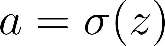 and activations
  , then returns two things: the
activations and a
, then returns two things: the
activations and a pullback closure. The pullback is the categorical
put-back. Given the upstream gradient from the layer above, it computes the
local gradient  , packs the
parameter gradients into a
, packs the
parameter gradients into a layer-grads (the outer product for dW, 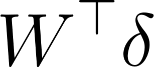 for
for db), and propagates  on to the previous layer. Because
the pullback is a closure, it remembers
on to the previous layer. Because
the pullback is a closure, it remembers 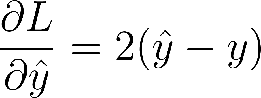 — that is what makes composing
lenses possible without storing every intermediate activation globally.
— that is what makes composing
lenses possible without storing every intermediate activation globally.
Now we can compose layers. network-forward walks the model’s layer list,
threading the current input and stacking pullbacks; the final output is the
scalar prediction (the XOR network has one output unit). Backpropagation,
model-backward, is literally the pullbacks composed in reverse order.
 1 ;; Forward pass through all layers, stacking pullbacks for reversal.
 2 (define (network-forward m xs)
 3   (let loop ([params-list (model-layers m)] [current-input xs] [pullbacks '()])
 4     (if (null? params-list)
 5         (values (car current-input) (reverse pullbacks))
 6         (let-values ([(acts pb) (forward-para (car params-list) sigmoid
 7                                               (compose sigmoid-deriv sigmoid)
 8                                               current-input)])
 9           (loop (cdr params-list) acts (cons pb pullbacks))))))
10
11 (define (mse-loss y-hat y)      (sqr (- y-hat y)))
12 (define (mse-loss-grad y-hat y) (* 2.0 (- y-hat y)))
13
14 ;; Backprop = compose the pullbacks in reverse order.
15 (define (model-backward pullbacks dl-dy)
16   (let go ([pbs (reverse pullbacks)] [upstream (list dl-dy)] [acc '()])
17     (if (null? pbs)
18         acc
19         (let-values ([(grads dx) ((car pbs) upstream)])
20           (go (cdr pbs) dx (cons grads acc))))))
21
22 ;; SGD update θ ← θ − η∇θ — an endomorphism on the model.
23 (define (update-layer params grads η)
24   (layer-params
25    (map (λ (wi dWi) (map (λ (w dw) (- w (* η dw))) wi dWi))
26         (layer-params-W params) (layer-grads-dW grads))
27    (map (λ (bi dbi) (- bi (* η dbi)))
28         (layer-params-b params) (layer-grads-db grads))))
29
30 (define (model-update m grads-list η)
31   (model (map (λ (p g) (update-layer p g η)) (model-layers m) grads-list)))
32
33 (define (train-step m xs y η)
34   (define-values (pred pullbacks) (network-forward m xs))
35   (values (model-update m (model-backward pullbacks (mse-loss-grad pred y)) η)
36           (mse-loss pred y)))
Note the one subtlety in model-backward: the loss gradient
 is a scalar, so it is
wrapped in a one-element list before entering the first pullback; every
pullback thereafter exchanges lists (activations and gradients are vectors).
This is the “covariant functor on the gradient category” from the theory
section:
is a scalar, so it is
wrapped in a one-element list before entering the first pullback; every
pullback thereafter exchanges lists (activations and gradients are vectors).
This is the “covariant functor on the gradient category” from the theory
section: 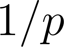 -vectors flow backward through exactly the same structure
the activations flowed forward through.
-vectors flow backward through exactly the same structure
the activations flowed forward through.
Training is then routine plumbing over this categorical spine: Glorot initialisation, network construction from an architecture spec, an SGD loop over epochs, and a predict function.
 1 (define (glorot fan-in fan-out)
 2   (define lim (sqrt (/ 6.0 (+ fan-in fan-out))))
 3   (- (* 2.0 lim (random)) lim))
 4
 5 (define (make-layer fan-in fan-out)
 6   (layer-params (for/list ([_ fan-out]) (for/list ([__ fan-in]) (glorot fan-in fan-out)))
 7                 (make-list fan-out 0.0)))
 8
 9 (define (make-network arch)
10   (model (map (λ (spec) (make-layer (car spec) (cadr spec))) arch)))
11
12 (define (train m dataset η epochs print-every)
13   (let loop ([cur m] [epoch 0])
14     (if (= epoch epochs)
15         cur
16         (let-values ([(m* total)
17                       (for/fold ([acc-m cur] [acc-loss 0.0]) ([pair dataset])
18                         (define-values (m** loss) (train-step acc-m (car pair) (cadr pair) η))
19                         (values m** (+ acc-loss loss)))])
20           (when (zero? (modulo epoch print-every))
21             (printf "  Epoch ~a  loss: ~a\n" epoch (~r total #:precision 6)))
22           (loop m* (add1 epoch))))))
23
24 (define (predict m xs)
25   (define-values (pred _) (network-forward m xs))
26   pred)
train folds one pass over the whole dataset per epoch: each example advances
the model (acc-m) and accumulates loss (acc-loss). Lazy Racket trivia: the
fold is a for/fold, which is tail-recursive because each iteration’s next
model state is produced by train-step before the loop continues.
II. Markov categories: stochastic morphisms
First, dropout as a stochastic lens. make-dropout-lens returns a function
that samples a Bernoulli mask, scales by  (inverted dropout keeps the
expected activation constant), and attaches a pullback that reuses the saved
mask. Both passes share the mask — that shared state is the stochastic
lens’s “closed optic” structure.
(inverted dropout keeps the
expected activation constant), and attaches a pullback that reuses the saved
mask. Both passes share the mask — that shared state is the stochastic
lens’s “closed optic” structure.
 1 ;; Dropout as a stochastic lens: the forward pass samples a Bernoulli(p)
 2 ;; mask, and the backward pass reuses the same mask (closed optic).
 3 (define (make-dropout-lens keep-prob)
 4   (λ (inputs)
 5     (define mask (for/list ([x inputs]) (if (< (random) keep-prob) 1.0 0.0)))
 6     (define scale (/ 1.0 keep-prob))
 7     (define (pullback upstream) (map (λ (u m) (* u m scale)) upstream mask))
 8     (values (map (λ (x m) (* x m scale)) inputs mask) pullback)))
 9
10 (define (gaussian-sample μ σ)              ; Box-Muller
11   (define u1 (+ 1e-10 (random)))
12   (define u2 (random))
13   (+ μ (* σ (sqrt (* -2.0 (log u1))) (cos (* 2.0 pi u2)))))
14
15 ;; Bayesian layer: W ~ N(μ, σ) sampled at each forward pass.
16 (struct bayesian-layer (mu sigma fan-out))
17
18 (define (make-bayesian-layer fan-in fan-out #:sigma [σ 0.1])
19   (bayesian-layer (for/list ([_ fan-out]) (for/list ([__ fan-in]) (glorot fan-in fan-out)))
20                   σ fan-out))
21
22 (define (bayesian-forward bl inputs)
23   (define σ (bayesian-layer-sigma bl))
24   (define W (map (λ (row) (map (λ (w) (gaussian-sample w σ)) row)) (bayesian-layer-mu bl)))
25   (map sigmoid (vec-add (matvec W inputs) (make-list (bayesian-layer-fan-out bl) 0.0))))
26
27 ;; Monte Carlo estimate of predictive mean and epistemic uncertainty.
28 (define (bayesian-predict-mc bl inputs n)
29   (define samples (for/list ([_ n]) (car (bayesian-forward bl inputs))))
30   (define mean (/ (apply + samples) n))
31   (values mean (sqrt (/ (apply + (map (λ (s) (sqr (- s mean))) samples)) n))))
The Bayesian layer stores the mean weight matrix  and a fixed spread
 . Each forward pass draws a fresh weight matrix
(via a Box-Muller transform), then
computes a sigmoid activation exactly like a deterministic layer would. The
Monte Carlo wrapper runs
. Each forward pass draws a fresh weight matrix
(via a Box-Muller transform), then
computes a sigmoid activation exactly like a deterministic layer would. The
Monte Carlo wrapper runs 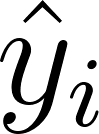 forward passes, returns their average as the
predictive mean, and their standard deviation as a measure of epistemic
uncertainty: high -estimate means the model is unsure about this
input.
forward passes, returns their average as the
predictive mean, and their standard deviation as a measure of epistemic
uncertainty: high -estimate means the model is unsure about this
input.
III. Invariance, equivariance, and k-means
Permutation-invariant pooling is one line: (apply + xs) — the colimit over
the set diagram, invariant because addition is commutative. The k-means
blocks read the same categorical way: update-centroids computes each cluster
centroid as the average (colimit) of its points, and nearest-centroid plays
the universal assignment morphism.
 1 ;; Σ xᵢ is the colimit over the set diagram — permutation-invariant by
 2 ;; commutativity of addition (basis of DeepSets).
 3 (define (permutation-invariant-pool xs) (apply + xs))
 4
 5 (define (euclidean-dist u v) (sqrt (apply + (map (λ (a b) (sqr (- a b))) u v))))
 6
 7 (define (nearest-centroid point centroids)
 8   (define dists (map (λ (c) (euclidean-dist point c)) centroids))
 9   (define min-d (apply min dists))
10   (for/first ([i (in-naturals)] [d dists] #:when (= d min-d)) i))
11
12 ;; K-means: each centroid is the colimit (average) of its cluster.
13 (define (update-centroids data labels k)
14   (for/list ([c (in-range k)])
15     (define cluster (for/list ([p data] [l labels] #:when (= l c)) p))
16     (if (null? cluster)
17         (make-list (length (car data)) 0.0)
18         (let ([n (length cluster)])
19           (map (λ (vs) (/ (apply + vs) n)) (apply map list cluster))))))
20
21 (define (k-means data k max-iter)
22   (let loop ([cents (take (shuffle data) k)] [iter 0])
23     (define labels (map (λ (p) (nearest-centroid p cents)) data))
24     (define new-cents (update-centroids data labels k))
25     (if (or (= iter max-iter) (equal? cents new-cents))
26         (values new-cents labels)
27         (loop new-cents (add1 iter)))))
update-centroids is worth a close read: for/list over the cluster index
 collects the points labelled into
 cluster; then
(apply map list cluster) transposes the list of points into a list of
coordinate columns, each averaged. An empty cluster (possible when  is
unlucky) falls back to the zero vector rather than crashing. The
is
unlucky) falls back to the zero vector rather than crashing. The k-means
loop alternates assignment and centroid update until centroids stop moving —
the fixed point is the categorical colimit structure in action.
IV. Topos: subobject classifier, sheaf gluing, Heyting algebra
subobject-classify is the characteristic morphism realized: it evaluates the
trained model to get the probability 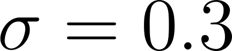 and
thresholds at to name the subobject.
and
thresholds at to name the subobject. sheaf-glue checks the
sheaf condition pairwise between all sections within tolerance and, if all
agree, returns the average — the glued global section. Failure to agree
returns #f, the categorical “no gluing”. The four Heyting operations are the
min/max/complement definitions from the theory section.
 1 ;; The sigmoid output IS the characteristic morphism χ : X → Ω; the
 2 ;; decision boundary is χ⁻¹(0.5).
 3 (define (subobject-classify model xs)
 4   (define prob (predict model xs))
 5   (values prob (if (>= prob 0.5) 1 0)))
 6
 7 (struct sheaf-section (context prediction))
 8
 9 ;; Glue local predictions into a global one iff all pairwise predictions
10 ;; agree within tol (the sheaf condition); #f means inconsistent.
11 (define (sheaf-glue sections tol)
12   (define n (length sections))
13   (define (consistent? i j)
14     (< (abs (- (sheaf-section-prediction (list-ref sections i))
15                (sheaf-section-prediction (list-ref sections j)))) tol))
16   (if (for*/and ([i (in-range n)] [j (in-range (add1 i) n)]) (consistent? i j))
17       (/ (apply + (map sheaf-section-prediction sections)) n)
18       #f))
19
20 ;; Ω carries a Heyting algebra (intuitionistic logic) — min/max/1−x.
21 (define (heyting-and p q)        (min p q))
22 (define (heyting-or  p q)        (max p q))
23 (define (heyting-not p)          (- 1.0 p))
24 (define (heyting-implies p q)    (heyting-or (heyting-not p) q))
V. Natural transformation: knowledge distillation
The distillation adapter is a linear map with sigmoid squashing: 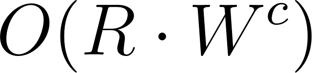 takes a teacher hidden representation and produces the student representation.
Because it is applied uniformly to any vector, it is a family of components
— exactly a natural transformation .
takes a teacher hidden representation and produces the student representation.
Because it is applied uniformly to any vector, it is a family of components
— exactly a natural transformation .
1 (struct nat-transform (adapter-W adapter-b))
2
3 (define (make-nat-transform source-size target-size)
4   (nat-transform (for/list ([_ target-size]) (for/list ([__ source-size]) (glorot source-size target-size)))
5                  (make-list target-size 0.0)))
6
7 (define (apply-nat-transform nt v)
8   (map sigmoid (vec-add (matvec (nat-transform-adapter-W nt) v) (nat-transform-adapter-b nt))))
The demo driver
The module+ main block seeds the random generator, then runs one demo per
perspective. It feeds the XOR dataset to the freshly built network, pushes a
vector through a dropout lens, queries the Bayesian layer 200 times, pools two
permutations of the same set, clusters the nine 2-D points, classifies the
trained XOR model, glues sheaf sections, evaluates Heyting formulas, and
distills a teacher’s hidden layer into a student representation.
 1 (module+ main
 2   (random-seed 42)
 3   (displayln "Category-Theory Deep Learning Framework in Racket")
 4   (displayln "Reference: Jia et al. (2025) Axioms 14(3):204")
 5
 6   ;; I. XOR via compositional backprop
 7   (displayln "\n== I. Para category + lens composition (XOR) ==")
 8   (define xor-data '(((0.0 0.0) 0.0) ((0.0 1.0) 1.0) ((1.0 0.0) 1.0) ((1.0 1.0) 0.0)))
 9   (define trained-xor (train (make-network '((2 4) (4 4) (4 1))) xor-data 0.5 6000 2000))
10   (for ([pair xor-data])
11     (define y-hat (predict trained-xor (car pair)))
12     (printf "  ~a -> target ~a, pred ~a, class ~a\n"
13             (car pair) (cadr pair) (~r y-hat #:precision 4) (if (> y-hat 0.5) 1 0)))
14
15   ;; II-A. Dropout as a stochastic lens
16   (displayln "\n== II. Markov categories ==")
17   (define-values (masked-vec pb-fn) ((make-dropout-lens 0.7) '(1.0 2.0 3.0 4.0 5.0)))
18   (printf "  dropout(0.7): ~a -> ~a\n" '(1.0 2.0 3.0 4.0 5.0)
19           (map (λ (x) (~r x #:precision 3)) masked-vec))
20   (printf "  grad (same mask): ~a\n"
21           (map (λ (x) (~r x #:precision 3)) (pb-fn '(1.0 1.0 1.0 1.0 1.0))))
22
23   ;; II-B. Bayesian layer, MC uncertainty
24   (define-values (μ-est σ-est)
25     (bayesian-predict-mc (make-bayesian-layer 3 1 #:sigma 0.3) '(1.0 0.5 -0.5) 200))
26   (printf "  Bayesian MC (200 samples): mean ~a, std ~a\n"
27           (~r μ-est #:precision 4) (~r σ-est #:precision 4))
28
29   ;; III-A. Permutation-invariant pooling
30   (displayln "\n== III. Invariance / equivariance ==")
31   (printf "  pool(1 3 5 2) = ~a, pool(3 1 2 5) = ~a (same result)\n"
32           (permutation-invariant-pool '(1.0 3.0 5.0 2.0))
33           (permutation-invariant-pool '(3.0 1.0 2.0 5.0)))
34
35   ;; III-B. K-means as colimit computation
36   (define cluster-data
37     '((1.0 1.0) (1.2 0.8) (0.9 1.1) (5.0 5.0) (5.1 4.9) (4.8 5.2) (1.0 5.0) (0.9 4.8) (1.1 5.1)))
38   (define-values (centroids labels) (k-means cluster-data 3 50))
39   (for ([c centroids] [i (in-naturals)])
40     (printf "  cluster ~a centroid: (~a, ~a)\n" i (~r (car c) #:precision 2) (~r (cadr c) #:precision 2)))
41   (printf "  labels: ~a\n" labels)
42
43   ;; IV-A. Subobject classifier on the trained XOR model
44   (displayln "\n== IV. Topos ==")
45   (for ([pair xor-data])
46     (define-values (prob cls) (subobject-classify trained-xor (car pair)))
47     (printf "  χ(~a) = ~a -> class ~a\n" (car pair) (~r prob #:precision 4) cls))
48
49   ;; IV-B. Sheaf gluing
50   (define s1 (sheaf-section "A" 0.72))
51   (define s2 (sheaf-section "B" 0.68))
52   (define s3 (sheaf-section "C" 0.91))
53   (printf "  glue A+B (tol 0.1): ~a\n"
54           (let ([g (sheaf-glue (list s1 s2) 0.1)]) (if g (~r g #:precision 4) "INCONSISTENT")))
55   (printf "  glue A+C (tol 0.1): ~a\n"
56           (let ([g (sheaf-glue (list s1 s3) 0.1)]) (if g (~r g #:precision 4) "INCONSISTENT")))
57
58   ;; IV-C. Heyting algebra
59   (printf "  Heyting: ~a ∧ ~a = ~a, ¬~a = ~a, ~a ⇒ ~a = ~a\n"
60           0.8 0.3 (heyting-and 0.8 0.3) 0.8 (heyting-not 0.8) 0.8 0.3 (heyting-implies 0.8 0.3))
61
62   ;; V. Natural transformation (teacher hidden → student)
63   (displayln "\n== V. Natural transformation (knowledge distillation) ==")
64   (define teacher-hidden
65     (let* ([layers (model-layers trained-xor)]
66            [l1 (list-ref layers 0)]
67            [l2 (list-ref layers 1)])
68       (define-values (a1 _pb1) (forward-para l1 sigmoid (compose sigmoid-deriv sigmoid) '(1.0 0.0)))
69       (define-values (a2 _pb2) (forward-para l2 sigmoid (compose sigmoid-deriv sigmoid) a1))
70       a2))
71   (printf "  teacher hidden: ~a\n" (map (λ (x) (~r x #:precision 4)) teacher-hidden))
72   (printf "  student rep:    ~a\n"
73           (map (λ (x) (~r x #:precision 4)) (apply-nat-transform (make-nat-transform 4 2) teacher-hidden))))
The distillation demo does something worth noticing: instead of re-running the
whole network, it invokes forward-para directly on the first two layers of
the trained model to harvest the 4-dimensional hidden representation — the
lens API pays for itself when you want access to intermediate structure, not
just the final prediction.
Running the code
From the directory containing the file, run:
1 racket deep_learning_category_theory.rkt
No packages beyond the standard Racket distribution are needed. Because of
random-seed 42 the output is fully reproducible and looks exactly like this:
 1 Category-Theory Deep Learning Framework in Racket
 2 Reference: Jia et al. (2025) Axioms 14(3):204
 3
 4 == I. Para category + lens composition (XOR) ==
 5   Epoch 0  loss: 1.173366
 6   Epoch 2000  loss: 0.002327
 7   Epoch 4000  loss: 0.000651
 8   (0.0 0.0) -> target 0.0, pred 0.0064, class 0
 9   (0.0 1.0) -> target 1.0, pred 0.9926, class 1
10   (1.0 0.0) -> target 1.0, pred 0.9888, class 1
11   (1.0 1.0) -> target 0.0, pred 0.0119, class 0
12
13 == II. Markov categories ==
14   dropout(0.7): (1.0 2.0 3.0 4.0 5.0) -> (1.429 2.857 0 5.714 0)
15   grad (same mask): (1.429 1.429 0 1.429 0)
16   Bayesian MC (200 samples): mean 0.3055, std 0.0717
17
18 == III. Invariance / equivariance ==
19   pool(1 3 5 2) = 11.0, pool(3 1 2 5) = 11.0 (same result)
20   cluster 0 centroid: (1.03, 0.97)
21   cluster 1 centroid: (1, 4.97)
22   cluster 2 centroid: (4.97, 5.03)
23   labels: (0 0 0 2 2 2 1 1 1)
24
25 == IV. Topos ==
26   χ((0.0 0.0)) = 0.0064 -> class 0
27   χ((0.0 1.0)) = 0.9926 -> class 1
28   χ((1.0 0.0)) = 0.9888 -> class 1
29   χ((1.0 1.0)) = 0.0119 -> class 0
30   glue A+B (tol 0.1): 0.7
31   glue A+C (tol 0.1): INCONSISTENT
32   Heyting: 0.8 ∧ 0.3 = 0.3, ¬0.8 = 0.19999999999999996, 0.8 ⇒ 0.3 = 0.3
33
34 == V. Natural transformation (knowledge distillation) ==
35   teacher hidden: (0.8588 0.0626 0.2403 0.0987)
36   student rep:    (0.3703 0.5728)
Interpreting the results
Run the program and read it as five little experiments, each confirming one categorical story.
I — the Para spine learned XOR, and the loss tells the story.
The epoch losses collapse from 1.173366 to 0.002327 to 0.000651 — a
steady exponential-ish decay with no divergence, which is what you expect from
compositional backprop on a well-posed problem. The real check is the
prediction table: (0,1) and (1,0) produce ~0.99 (class 1), while (0,0)
and (1,1) produce ~0.01 (class 0). XOR is not linearly separable, so a
network that nails it proves the lens composition is actually computing two
nonlinear feature layers correctly, not just memorizing thresholds. The small
residual (0.0064 vs. a perfect 0) is sigmoid saturation slack, nothing more.
II — dropout and Bayesian layers behave as stochastic morphisms.
Of the five activations, elements 3 and 5 were dropped to 0; the survivors were rescaled by  :
: 1.0 \to 1.429, 2.0 \to 2.857, 4.0 \to 5.714. The backward pass returns the same mask multiplied by the same scale — (1.429 1.429 0 1.429 0) — which is the closed-optic requirement made visible: no gradient flows through dropped units, and surviving gradients are rescaled so updates stay unbiased. The Bayesian MC query returns mean 0.3055, std 0.0717: the sigmoid-squashed predictions spread by a standard deviation of ~0.07 around 0.31, which quantifies how much the weight noise  actually matters for this input. A confident model would report a much smaller std.
III — invariance and colimits are visible in two lines.
Both permutations of the set {1,3,5,2} pool to 11.0: the colimit ignores
order by construction. K-means finds the structure we planted: centroids
(1.03, 0.97), (1, 4.97), (4.97, 5.03) — within ~0.05 of the true cluster
means (1,1), (1,5), (5,5). The labels (0 0 0 2 2 2 1 1 1) are exact:
each of the three planted clusters is recovered with zero misassignments. The
centroid-as-colimit reading is not a metaphor here; it is literally how the
code computes them (average of the cluster’s points).
IV — the topos logic behaves exactly like set-theoretic logic.
The trained classifier’s χ readings mirror the XOR table: high probabilities
(membership) on the two positive points, low on the two negative ones, and
class thresholds at χ⁻¹(0.5) agree with the raw predictions. The sheaf
gluing is the most instructive line: A+B (0.72 vs. 0.68, difference 0.04 <
0.1) glue into 0.7 — the average — while A+C (0.72 vs. 0.91, difference
0.19 ≥ 0.1) refuse to glue: inconsistent experts are flagged rather than
silently averaged, which is the sheaf condition protecting you from
ensembling disagreeing models. The Heyting line demonstrates the
[0,1]-valued logic: 0.8 ∧ 0.3 = 0.3, ¬0.8 = 0.1999... (float arithmetic
shows its 0.2 as 0.19999999999999996 — harmless), and implication
0.8 ⇒ 0.3 = max(0.2, 0.3) = 0.3.
V — distillation compresses the teacher’s representation.
The teacher hidden vector for input (1.0, 0.0) is 4-dimensional:
(0.8588 0.0626 0.2403 0.0987) — mostly-concentrated feature activity with one
dominant unit. The student adapter squeezes it to 2 dimensions: (0.3703 0.5728). The
point of the demo is not that these numbers are meaningful on their own; it is
that is a uniform map — apply the same adapter to any teacher hidden
state and you get a comparable student state, which is the naturality condition
making distillation a bona fide natural transformation rather than a hand-fitted
regression.
Summary
Category theory gave us a vocabulary, and the vocabulary gave us structure.
The five sections of the file are five named categorical constructions: layers
are Para morphisms and lenses, dropout and Bayesian layers are stochastic
morphisms in a Markov category, pooling and k-means compute colimits,
classification is characteristic map into with sheaf-conditioned
ensembling, and distillation is a natural transformation. Each one compressed
into a few lines of Racket that would otherwise be an ad hoc engineering
special case — and each one carries the laws of its construction for free.
The complete framework is about 285 lines and uses only the standard Racket
distribution. To explore further: replace sigmoid with ReLU (and its
derivative), try deeper architectures by editing the make-network spec, or
widen the dropout lens into an input-space perturbator — the categorical
scaffolding does not change, only the morphisms you plug in.