Tree Diagrams
What is a Tree Diagram?
The ‘Tree layout’ is not a distinct type of diagram per se. Instead, it’s representative of D3’s family of hierarchical layouts.
It’s designed to produce a ‘node-link’ diagram that lays out the connection between nodes in a method that displays the relationship of one node to another in a parent-child fashion.
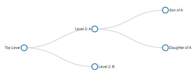
For example, the following diagram shows a root node (the starting position) labelled ‘Top Node’ which has two children (Bob: Child of Top Node and Sally: Child of Top Node). Subsequently, Bob:Child of Top Node has two dependant nodes (children) ‘Son of Bob’ and ‘Daughter of Bob’.
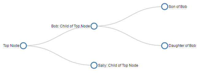
The clear advantage to this style of diagram is that describing it in text is difficult, but representing it graphically makes the relationships easy to determine.
The data required to produce this type of layout needs to describe the relationships, but this is not necessarily an onerous task. For example, the following is the data (in JSON form) for the diagram above and it shows the minimum information required to form the correct layout hierarchy.
It shows each node as having a name that identifies it on the tree and, where appropriate, the children it has (as an array).
There is a wealth of examples of tree diagrams on the web, but I would recommend a visit to blockbuilder.org as a starting point to get some ideas.
In this chapter we’re going to look at a very simple piece of code to generate a tree diagram before looking at different ways to adapt it. Including rotating it to be vertical, adding some dynamic styling to the nodes, importing from a flat file and from an external source. Finally we’ll look at a more complex example that is more commonly used on the web that allows a user to expand and collapse nodes interactively.
A simple Tree Diagram explained
We are going to work through a simple example of the code that draws a tree diagram, This is more for the understanding of the process rather than because it is a good example of code for drawing a tree diagram. It is a very limited example that lacks any real interactivity which is one of the strengths of d3.js graphics. However, we will outline the operation of an interactive version towards the end of the chapter once we have explored some possible configuration options that we might want to make.
The graphic that we are going to generate will look like this…
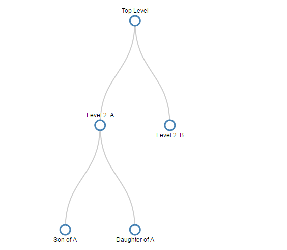
The full code for it looks like this;
<!DOCTYPE html>
<meta charset="utf-8">
<style> /* set the CSS */

.node circle {
  fill: #fff;
  stroke: steelblue;
  stroke-width: 3px;
}

.node text { font: 12px sans-serif; }

.node--internal text {
  text-shadow: 0 1px 0 #fff, 0 -1px 0 #fff, 1px 0 0 #fff, -1px 0 0 #fff;
}

.link {
  fill: none;
  stroke: #ccc;
  stroke-width: 2px;
}

</style>

<body>

<!-- load the d3.js library -->
<script src="//d3js.org/d3.v4.min.js"></script>
<script>

var treeData =
  {
    "name": "Top Level",
    "children": [
      {
		"name": "Level 2: A",
        "children": [
          { "name": "Son of A" },
          { "name": "Daughter of A" }
        ]
      },
      { "name": "Level 2: B" }
    ]
  };

// set the dimensions and margins of the diagram
var margin = {top: 40, right: 30, bottom: 50, left: 30},
    width = 660 - margin.left - margin.right,
    height = 500 - margin.top - margin.bottom;

// declares a tree layout and assigns the size
var treemap = d3.tree()
    .size([width, height]);

//  assigns the data to a hierarchy using parent-child relationships
var nodes = d3.hierarchy(treeData);

// maps the node data to the tree layout
nodes = treemap(nodes);

// append the svg obgect to the body of the page
// appends a 'group' element to 'svg'
// moves the 'group' element to the top left margin
var svg = d3.select("body").append("svg")
      .attr("width", width + margin.left + margin.right)
      .attr("height", height + margin.top + margin.bottom),
    g = svg.append("g")
      .attr("transform",
            "translate(" + margin.left + "," + margin.top + ")");

// adds the links between the nodes
var link = g.selectAll(".link")
    .data( nodes.descendants().slice(1))
  .enter().append("path")
    .attr("class", "link")
    .attr("d", function(d) {
       return "M" + d.x + "," + d.y
         + "C" + d.x + "," + (d.y + d.parent.y) / 2
         + " " + d.parent.x + "," +  (d.y + d.parent.y) / 2
         + " " + d.parent.x + "," + d.parent.y;
       });

// adds each node as a group
var node = g.selectAll(".node")
    .data(nodes.descendants())
  .enter().append("g")
    .attr("class", function(d) {
      return "node" +
        (d.children ? " node--internal" : " node--leaf"); })
    .attr("transform", function(d) {
      return "translate(" + d.x + "," + d.y + ")"; });

// adds the circle to the node
node.append("circle")
  .attr("r", 10);

// adds the text to the node
node.append("text")
  .attr("dy", ".35em")
  .attr("y", function(d) { return d.children ? -20 : 20; })
  .style("text-anchor", "middle")
  .text(function(d) { return d.data.name; });

</script>
</body>
In the course of describing the operation of the file I will gloss over the aspects of the structure of an HTML file which have already been described at the start of the book. Likewise, aspects of the JavaScript functions that have already been covered will only be briefly explained.
The start of the file deals with setting up the document’s head and body loading the d3.js script and setting up the CSS in the <style> section.
The CSS section sets styling for the circle that represents the nodes, the text alongside them and the links between them.
.node circle {
  fill: #fff;
  stroke: steelblue;
  stroke-width: 3px;
}

.node text { font: 12px sans-serif; }

.node--internal text {
  text-shadow: 0 1px 0 #fff, 0 -1px 0 #fff, 1px 0 0 #fff, -1px 0 0 #fff;
}

.link {
  fill: none;
  stroke: #ccc;
  stroke-width: 2px;
}
Then our JavaScript section starts and the first thing that happens is that we declare our array of data in the following code;
var treeData =
  {
    "name": "Top Level",
    "children": [
      {
		"name": "Level 2: A",
        "children": [
          { "name": "Son of A" },
          { "name": "Daughter of A" }
        ]
      },
      { "name": "Level 2: B" }
    ]
  };
As outlined at the start of the chapter, this data is encoded hierarchically in JavaScript Object Notation (JSON). Each node must have a name and if it is going to have subordinate nodes it must include a ‘children’ element. There are many examples of hierarchical data that can be encoded in this way. From the traditional parent - offspring example to directories on a hard drive or a breakdown of materials for a complex object. Any system of encoding where there is a single outcome from multiple sources like an election or an alert encoding system dependent on multiple trigger points.
The next section of our code declares some of the standard features for our diagram such as the size and shape of the svg container with margins included.
// set the dimensions and margins of the diagram
var margin = {top: 40, right: 90, bottom: 50, left: 90},
    width = 660 - margin.left - margin.right,
    height = 500 - margin.top - margin.bottom;
Now we start to get into the specifics for the diagram. The next block of code invokes the D3 .tree component, configures the data and assigns it to the tree structure (no actual drawing mind you, just getting the data ready).
// declares a tree layout and assigns the size
var treemap = d3.tree()
    .size([width, height]);

//  assigns the data to a hierarchy using parent-child relationships
var nodes = d3.hierarchy(treeData);

// maps the node data to the tree layout
nodes = treemap(nodes);
The first part of this is the declaration of treemap as using the d3.tree function and assigning the size of the diagram from our earlier variables;
// declares a tree layout and assigns the size
var treemap = d3.tree()
    .size([width, height]);
Then we assign our data (with the variable treeData) to nodes using the d3.hierarchy function.
//  assigns the data to a hierarchy using parent-child relationships
var nodes = d3.hierarchy(treeData, function(d) {
    return d.children;
  });
This assigns a range of properties to each node including;
-
node.data- the data associated with the node (in our case it will include the name accessible asnode.data.name) -
node.depth- a representation of the depth or number of hops from the initial ‘root’ node. -
node.height- the greatest distance from any descendant leaf nodes -
node.parent- the parent node, or null if it’s the root node -
node.children- child nodes or undefined for any leaf nodes
While we’re telling the function to use the ‘children’ elements from ‘treeData’, to generate the properties for the nodes, by default it will use the name ‘children’ if a name is not specified.
Lastly for this block we map the ‘nodes’ data to the tree layout;
// maps the node data to the tree layout
nodes = treemap(nodes);
The next block of code appends our SVG working area to the body of our web page and creates a group element (<g>) that will contain our svg objects (our nodes, text and links).
var svg = d3.select("body").append("svg")
      .attr("width", width + margin.left + margin.right)
      .attr("height", height + margin.top + margin.bottom),
    g = svg.append("g")
      .attr("transform",
            "translate(" + margin.left + "," + margin.top + ")");
Now we’re going to start drawing something! First up is the trickiest part. The links between the nodes.
// adds the links between the nodes
var link = g.selectAll(".link")
    .data( nodes.descendants().slice(1))
  .enter().append("path")
    .attr("class", "link")
    .attr("d", function(d) {
       return "M" + d.x + "," + d.y
         + "C" + d.x + "," + (d.y + d.parent.y) / 2
         + " " + d.parent.x + "," +  (d.y + d.parent.y) / 2
         + " " + d.parent.x + "," + d.parent.y;
       });
I say tricky because we’re going to be using the svg mini language again, and while it will work just fine if we simply paste it in and move on, if we want to understand a bit more about how it works, we will need to take a bit of a detour.
But first we need to get the details for this block of code explained. We declare and select all the ‘links’ and then assign the nodes as ‘data’ (.data(nodes.descendants().slice(1))). When we do this we are using .descendants() to return the array of ‘descendant’ nodes. We also specify .slice(1) to not include the main ‘root’ node since the links will be drawn by drawing a line from a child node to its parent (which we wouldn’t be able to do with the root node).
We append a path (.enter().append("path")) and apply some styling (.attr("class", "link")) and then embark on drawing the link lines with the SVG mini language via the ‘d’ attribute.
As we have mentioned previously the ‘d’ attribute allows for the creation of a string of instructions that describe a path. These instructions include;
- Moveto : moves the drawing point using
Mfor absolute coordinates andmfor relative movements - Lineto : draws a straight line from the current position to the next specified location using
Lfor absolute coordinates andlfor relative movement. - Curveto : draws a Bezier curve using control points from the current position to an end point.
Cdesignates absolute coordinates andcis used for relative movement. Either one or two sets of control points are used depending on whether a quadratic or cubic Bezier curve is used. - Arcto : describes a curved path as an elliptical curve rather than a Bezier with additional complexity
- ClosePath : draws a straight line from the current position to the first point in the path
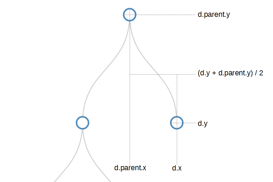
If we look at a single node instance and break down the ‘d’ attribute path we can see the following;
-
"M" + d.x + "," + d.y: Moves to the starting point of our node -
"C" + d.x + "," + (d.y + d.parent.y) / 2: Establishes that we are going to draw a Cubic (C) Bezier curve and the first control point for it is atd.xin the x dimension and halfway between the starting node and its parent. -
" " + d.parent.x + "," + (d.y + d.parent.y) / 2: Sets the second control point for the curve in line with the parent node in the x dimension and still halfway between the starting node and its parent in the y dimension. -
" " + d.parent.x + "," + d.parent.y: sets the end point for our curve at the parent node location.
If we wanted to make the code easier to follow we could change the curve between nodes to a straight line with the following code;
// adds the links between the nodes
var link = g.selectAll(".link")
    .data( nodes.descendants().slice(1))
  .enter().append("path")
    .attr("class", "link")
    .attr("d", function(d) {
       return "M" + d.x + "," + d.y
         + "L" + d.parent.x + "," + d.parent.y;
       });
Which would result in lines being drawn with coordinates from the ‘d’ attribute as follows;
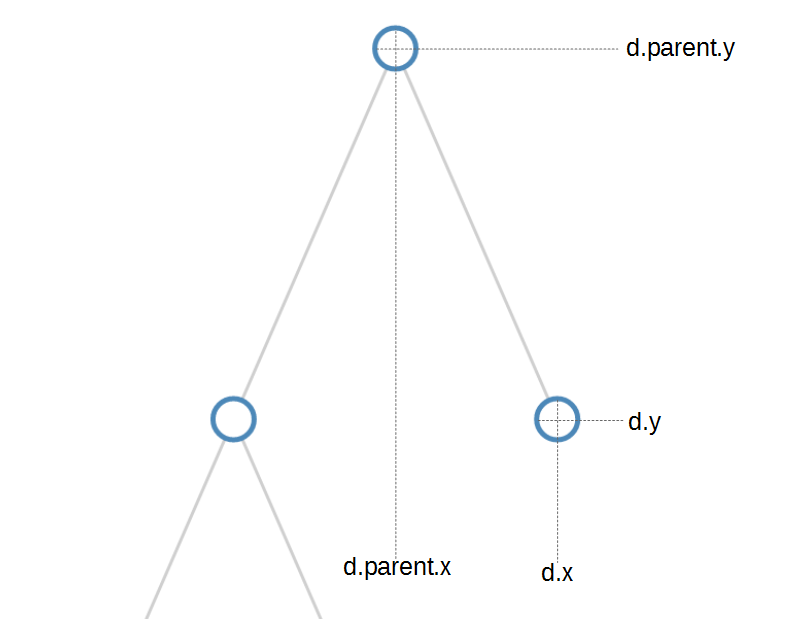
Then we create a variable node that creates a group element (g) for each node;
// adds each node as a group
var node = g.selectAll(".node")
    .data(nodes.descendants())
  .enter().append("g")
    .attr("class", function(d) {
      return "node" +
        (d.children ? " node--internal" : " node--leaf"); })
    .attr("transform", function(d) {
      return "translate(" + d.x + "," + d.y + ")"; });
This time we can see that;
- We don’t slice off the root node (
.data(nodes.descendants())) from our data set. - We apply a different ‘class’ to the node depending on whether it’s an internal node (it has children) or it’s a leaf node (it has no children)
d.children ? " node--internal" : " node--leaf". - We place each node ‘group’ at the appropriate location.
- We don’t actually draw anything. All we’re doing is getting the properties for each node set.
Once we have everything set up we can start to add objects to our node groups.
First we add our circle;
// adds the circle to the node
node.append("circle")
  .attr("r", 10);
And then we add the text;
// adds the text to the node
node.append("text")
  .attr("dy", ".35em")
  .attr("y", function(d) { return d.children ? -20 : 20; })
  .style("text-anchor", "middle")
  .text(function(d) { return d.data.name; });
When we’re adding the text, we make sure that we add it on the side appropriate for either a leaf node or an internal node.
And there’s our tree diagram.
A horizontal tree diagram explained
As we discussed at the start of the previous section, we wanted to start describing tree diagrams with a vertical version because there was an added degree of complexity with the horizontal version that might cause some confusion. If you have worked through and understood the vertical version, the horizontal won’t present any problems other than when you go “Oh, I see what’s going on.”. If you find yourself part way through this description of the changes to the code and can’t see what’s going on, revisit the vertical code and come back.
The graphic that we are going to generate will look like this…
The full code for this is almost identical to the code for the vertical tree diagram with a couple of simple, yet major changes.
The first change is that the way that we draw the diagram relies on changing our reference by rotating everything by 90 degrees.
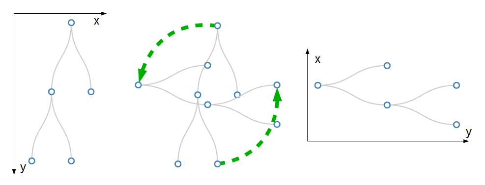
The (very simplistic) diagram shows that what used to be our ‘x’ dimension is now our ‘y’ dimension and visa versa.
The second change is that where we rotated our axes above we are now left with y and x dimensions that have an origin in the bottom left of the graph. Of course when we draw our diagram, the origin is in the top left corner. This vertical flip occurs automatically and is the reason the diagram doesn’t appear to have ‘just’ rotated.
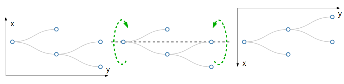
Now we have our origin in the top left again and the layout of our tree looks pretty much as the example we will be producing.
Believe it or not, this is WAY more difficult to explain than it is to actually do. Again, D3 takes care of the heavy lifting, the explanation of the changes above is just to help us understand why we make some of the changes.
The first change we make is just to give ourselves some extra margin space since some of the labels extend slightly more left and right with a horizontal diagram;
var margin = {top: 20, right: 90, bottom: 30, left: 90},
The second change sets the size of the graphic. Here the width and height are swapped as part of the rotation.
// declares a tree layout and assigns the size
var treemap = d3.tree()
    .size([height, width]);
When we add the links we need to incorporate the rotation and the easiest way to appreciate the change is to compare the two pieces of code at the same time. In fact it is only when we draw the ‘d’ attribute for the path that we see the changes.
Firstly the vertical tree code;
    .attr("d", function(d) {
       return "M" + d.x + "," + d.y
         + "C" + d.x + "," + (d.y + d.parent.y) / 2
         + " " + d.parent.x + "," +  (d.y + d.parent.y) / 2
         + " " + d.parent.x + "," + d.parent.y;
       });
Then the horizontal tree code;
    .attr("d", function(d) {
       return "M" + d.y + "," + d.x
         + "C" + (d.y + d.parent.y) / 2 + "," + d.x
         + " " + (d.y + d.parent.y) / 2 + "," + d.parent.x
         + " " + d.parent.y + "," + d.parent.x;
       });
While there is a bit of math involved, the easiest way to tell that there is a difference is that for the horizontal tree, each coordinate is being described in y,x fashion rather than the conventional x,y.
A similar coordinate change is made when we translate the positions for the nodes;
    .attr("transform", function(d) {
      return "translate(" + d.y + "," + d.x + ")"; });
And lastly when we place the text next to the circles we need to adjust the default ‘y’ distance value with an ‘x’ distance value and to ensure that the labels are spaced at an appropriate distance and to align the text to either the left or right depending on whether it has children or not. We adjust the text anchor appropriately with an ‘end’ or ‘start’.
node.append("text")
  .attr("dy", ".35em")
  .attr("x", function(d) { return d.children ? -13 : 13; })
  .style("text-anchor", function(d) {
    return d.children ? "end" : "start"; })
  .text(function(d) { return d.data.name; });
And there we are….
The full code for this example can be found on github, or in the code samples bundled with this book (simple-horizontal-tree-diagram.html). A working example can be found on bl.ocks.org.
Styling nodes in a tree diagram
Changing node and link colours
The nodes in a tree diagram are objects that exist to provide a representation of the structure of data, but on a tree diagram they should also be viewed as an opportunity to encode additional information about the underlying data.
From the horizontal example shown we have encoded a certain amount of information already. The position of the text relative to each node is determined by whether or not the node is the parent of another node (if it’s a parent it’s on the left) or a child that is on the edge of the tree (in which case it is on the right of the node).
Now, that’s nice, but are we going to be satisfied with that??? (The answer is “No” by the way.)
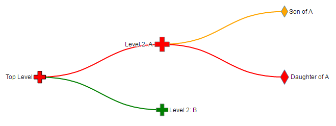
This example is fairly simple, but it is an example of applying different styles to the nodes to convey additional information. I should be clear at this stage that I am not advocating turning your tree diagram into something that looks like it came out of a circus, because that would be a crime against style, so don’t repeat my upcoming example, but let some of the features be a trigger for developing your own subtle, yet compelling visualizations.
Brace yourself. Here’s a picture of the tree diagram that we’re going to generate. Those with weaker constitutions should look away and flip forward a few pages;
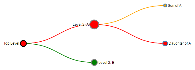
The changes that have been made are as a result of additional data fields that have been added to the JSON array and these fields have been applied to various style options throughout the code.
The types of style changes we have made are - Variation of the diameter of nodes - Changing the fill and stroke colour of nodes - Changing the colour of links depending on the associated node they are connected to.
The code changes we describe from here are assuming that we start with our simple horizontal tree diagram from the previous chapter. We’ll start by looking at the new JSON data set;
Each node now has a value which might represent a degree of importance (we will use this to affect the radius of the nodes), a type which might indicate a difference in the type of node (they might be in active, inactive or undetermined states) and a level which might indicate an alert level for determining problems (red = bad, orange = caution and green = normal).
Irrespective of the contrived nature of our styling options, they are applied to our tree in fairly similar ways with some subtle differences.
The full code for this example can be found on github or in the code samples bundled with this book (tree-styling.html). A working example can be found on bl.ocks.org.
The first change is to the node radius, stroke colour and fill colour.
We simply change the portion of the code that appends the circle from this…
// adds the circle to the node
node.append("circle")
  .attr("r", 10);
… to this …
// adds the circle to the node
node.append("circle")
  .attr("r", function(d) { return d.data.value; })
  .style("stroke", function(d) { return d.data.type; })
  .style("fill", function(d) { return d.data.level; });
The changes return the radius attribute as a function using data.value, the stroke colour is returned using data.type and the fill colour is returned with data.level. This is nice and simple, but we do need to make a slight adjustment to the code that sets the distance that the text is from the nodes so that when the radius expands or contracts, the text distance from the edge of the node adjusts as well.
To do this we take the clever piece of code that adjusts the distance that the text is in the x dimension from the node that looks like this …
.attr("x", function(d) { return d.children ? -13 : 13; })
… and we add in a dynamic aspect using the data.value field.
  .attr("x", function(d) { return d.children ?
    (d.data.value + 4) * -1 : d.data.value + 4 })
The last thing we wanted to do is to change the colour of the link based on the colour of the node. We accomplish this by taking the code that inserts the links…
// adds the links between the nodes
var link = g.selectAll(".link")
    .data( nodes.descendants().slice(1))
  .enter().append("path")
    .attr("class", "link")
    .attr("d", function(d) {
       return "M" + d.y + "," + d.x
         + "C" + (d.y + d.parent.y) / 2 + "," + d.x
         + " " + (d.y + d.parent.y) / 2 + "," + d.parent.x
         + " " + d.parent.y + "," + d.parent.x;
       });;
… and adding in a line that styles the link colour (the stroke) based on the data.level colour of node.
// adds the links between the nodes
var link = g.selectAll(".link")
    .data( nodes.descendants().slice(1))
  .enter().append("path")
    .attr("class", "link")
    .style("stroke", function(d) { return d.data.level; })
    .attr("d", function(d) {
       return "M" + d.y + "," + d.x
         + "C" + (d.y + d.parent.y) / 2 + "," + d.x
         + " " + (d.y + d.parent.y) / 2 + "," + d.parent.x
         + " " + d.parent.y + "," + d.parent.x;
       });
Use the concepts here wisely. I don’t want to see any heinously styled tree diagrams floating around the internet with “Thanks to the help from D3 Tips and Tricks” next to them. Be subtle, be thoughtful :-).
Changing the nodes to different shapes
Many thanks to Josiah who asked a question on the d3noob.org blog on how the shapes of the nodes could be varied based on an associated value in the data.
There is more than one way to do this, but perhaps the simplest is to replace the section of the JavaScript that appends the circle with one that appends a symbol from d3’s symbol generator.
There are six pre-defined symbol types as follows;
- circle (
d3.symbolCircle) - a circle. - cross (
d3.symbolCross) - a Greek cross or plus sign. - diamond (
d3.symbolDiamond) - a rhombus. - square (
d3.symbolSquare) - an axis-aligned square. - triangle (
d3.symbolTriangle) - an upward-pointing equilateral triangle. - star (
d3.symbolStar) - a five pointed star. - ‘Y’ (
d3.symbolWye) - a ‘Y’ shape.
If we start with our ‘tree-styling’ script from above we can replace the code block that added the circles with the following script will look at the value in the data and assign either a cross or a diamond depending on the value
// adds symbols as nodes
node.append("path")
  .style("stroke", function(d) { return d.data.type; })
  .style("fill", function(d) { return d.data.level; })
  .attr("d", d3.symbol()
     .size(function(d) { return d.data.value * 30; } )
     .type(function(d) { if
       (d.data.value >= 9) { return d3.symbolCross; } else if
       (d.data.value <= 9) { return d3.symbolDiamond;}
     }));
It will also adjust the size of the symbol along with the stroke and fill.
The full code for this example can be found on github or in the code samples bundled with this book (tree-symbol.html). A working online example can be found on bl.ocks.org.
Using images as nodes
Many thanks to nbhatta who asked a question on the d3noob.org blog on how to use images as nodes.
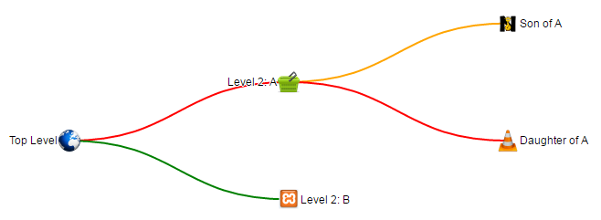
This was a slightly simpler change and just involved replacing the code snippet that added the circles with one that added an image;
// adds images as nodes
node.append("image")
  .attr("xlink:href", function(d) { return d.data.icon; })
  .attr("x", "-12px")
  .attr("y", "-12px")
  .attr("width", "24px")
  .attr("height", "24px");
The images I chose were all 48 x 48 pixel for the sake of consistency and in the code above I formatted them to be half that size and moved them in the x and y direction so that they were centred correctly.
The cool thing that you will notice is that the specific icon that is placed at each node position is set by the name of the icon which is gathered from the JSON file with the tree details;
var treeData =
  {
    "name": "Top Level",
    "value": 10,
    "type": "black",
    "level": "red",
    "icon": "earth.png",
    "children": [
      {
        "name": "Level 2: A",
        "value": 5,
        "type": "grey",
        "level": "red",
       "icon": "cart.png",
        "children": [
          {
            "name": "Son of A",
            "value": 5,
            "type": "steelblue",
            "icon": "lettern.png",
            "level": "orange"
          },
          {
            "name": "Daughter of A",
            "value": 18,
            "type": "steelblue",
            "icon": "vlc.png",
            "level": "red"
          }
        ]
      },
      {
        "name": "Level 2: B",
        "value": 10,
        "type": "grey",
        "icon": "random.png",
        "level": "green"
      }
    ]
  };
It’s possible to just have a single image and to hard-code it into the script, but where’s the fun in that?
The full code for this example can be found on github or in the code samples bundled with this book (tree-images.html, cart.png, earth.png, lettern.png, random.png and vlc.png). A working online example can be found on bl.ocks.org.
Generating a tree diagram from external data
In all the examples we have looked at so far we have used data that we have declared from within the file itself. Being able to import data from an external file is an important feature that we need to know how to implement.
Starting from the simple tree diagram example that we began with at the start of the chapter, the first change that we need to make is to remove the section of code that declares our data. But don’t throw it away since we will use it to create a separate file called treeData.json. Its contents will be;
(don’t include the treeData = part, or the semicolon at the end (you can delete those))
Then all we need to do is include a section that uses the d3.json accessor to load the file treeData.json (Remember to correctly address the file. This one assumes that the treeData.json file is in the same directory as the html file we are opening).
// load the external data
d3.json("treeData.json", function(error, treeData) {
if (error) throw error;
We can put it somewhere near the start of the JavaScript, but make sure it comes before the ‘nodes’ declaration (when in doubt, check out the sample code).
We also need to make sure that we include the wrapping, closing curly braces and bracket / semicolon (});) at the end of the script.
The full code for this example can be found on github or in the code samples bundled with this book (tree-from-external.html and treeData.json). A working example can be found on bl.ocks.org.
Generating a tree diagram from ‘flat’ data
Tree diagrams are a fantastic way of displaying information, but one of the drawbacks (to the examples we’ve been using so far) is the need to have your data encoded hierarchically. Most data in a raw form will be flat. That is to say, it won’t be formatted as an array with the parent - child relationships. Instead it will be a list of objects (which we will want to turn into nodes) that might describe the relationship to each other, but they won’t be encoded that way. For example, the following is the flat representation of the example data we have been using thus far.
It is actually fairly simple and consists of only the name of the node and the name of its parent node. It’s easy to see how this data could be developed into a hierarchical form, but it would take a little time and for a larger data set, that would be tiresome.
Luckily computers are built for shuffling data about and with the advent of v4 of d3.js we now have the d3.stratify operator that will convert flat data into a hierarchy suitable for use in our tree diagram.
We will be using the simple example that we started with at the start of the chapter and the first change we need to make is to replace our original data…
var treeData =
{
  "name": "Top Level",
  "children": [
    {
      "name": "Level 2: A",
      "children": [
        { "name": "Son of A" },
        { "name": "Daughter of A" }
      ]
    },
    { "name": "Level 2: B" }
  ]
};
… with our flat data array…
var flatData = [
  {"name": "Top Level", "parent": null},
  {"name": "Level 2: A", "parent": "Top Level" },
  {"name": "Level 2: B", "parent": "Top Level" },
  {"name": "Son of A", "parent": "Level 2: A" },
  {"name": "Daughter of A", "parent": "Level 2: A" }
];
It’s worth noting here that we have also changed the name of the array (to flatData) since we are going to convert, then declare our newly massaged data with our original variable name treeData so that the remainder of our code thinks there have been no changes.
Then we use the d3.stratify operator on our flat data;
// convert the flat data into a hierarchy
var treeData = d3.stratify()
  .id(function(d) { return d.name; })
  .parentId(function(d) { return d.parent; })
  (flatData);
The stratify function requires a unique identifier to be used for each node and it will be declared as .id. In this example each of our nodes has a unique ‘name’, so we are using that as our id (.id(function(d) { return d.name; })). We also need to understand the hierarchy by having each node identify who its parent is. This will be stored as parentId (.parentId(function(d) { return d.parent; }))
That’s it!
Because we want to be able to use our code as intact as possible from our horizontal tree example we will want to run through our dataset and assign the ‘name’ to each node that has been stored as id;
// assign the name to each node
treeData.each(function(d) {
    d.name = d.id;
  });
That’s it!
The brevity of the code to do this is fantastic and well done to Mike Bostock for including the new function in v4. Of course, the end result looks exactly the same;
… but it adds a significant capability for use of additional data.
The full code for this example can be found on github or in the code samples bundled with this book (tree-from-flat.html). A working example can be found on bl.ocks.org.
Generating a tree diagram from a CSV file.
Creating a tree diagram from a csv file is an extension of the sections where we create a diagram from flat data and where we create a diagram from an external file.
By mashing these together and using a csv file something like the following…
… we can ingest the name of the nodes and their relationships and then format the data correctly.
The main piece of code that we would add that is different from the standard horizontal tree diagram is as follows;
// load the external data
d3.csv("treeCsv.csv", function(error, flatData) {
  if (error) throw error;

  // assign null correctly
  flatData.forEach(function(d) {
      if (d.parent == "null") { d.parent = null};
    });

  // convert the flat data into a hierarchy
  var treeData = d3.stratify()
    .id(function(d) { return d.name; })
    .parentId(function(d) { return d.parent; })
    (flatData);

  // assign the name to each node
  treeData.each(function(d) {
      d.name = d.id;
    });
The only part of that code which is new is the portion where we look for the node whose parent is ‘“null”’ and change it to null. This is necessary since the script interprets the name as actually being the text ‘null’ so we have to force the code to realise that we want it to refer to a null amount.
The end result looks very familiar.
The full code for this example can be found on github or in the code samples bundled with this book (tree-from-csv.html and treeCsv.csv). A working example can be found on bl.ocks.org.
An interactive tree diagram
The examples presented thus far have all been static in the sense that they present information on a web page, but that’s where they stop. One of the strengths of web content is the ability to involve the reader to a greater extent. Therefore the following tree diagram example includes an interactive element where the user can click on any parent node and it will collapse on itself to make more room for others or to simplify a view. Additionally, any collapsed parent node can be clicked on and it will re-grow to its previous condition.
The example included here has it’s roots in the is v3 tree diagram of Mike Bostock’s example. Kudos and thanks also go out to Soumya Ranjan for steering me in the fight direction for the diagonal solution. This was necessary to work around the deprecation of svg.diagonal in v3.
The full code for this example can be found on github, in the appendices of this book or in the code samples bundled with this book (interactive-tree.html). A working online example can be found on bl.ocks.org.
For a brief visual description of the action. The diagram will initially display a partially collapsed tree…
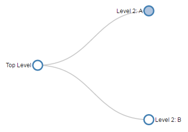
Then when clicking on the ‘Level 2: A’ node, the tree expands to…
We could also click on the root node (`Top Level’) to fully collapse the tree…

Then clicking on the nodes opens the diagram back up again.
One of the important changes is to allow the diagram to follow the d3.js model of enter - update - exit for the nodes with a suitable transition in between.
Nodes are coloured (“steelblue”) if they have been collapsed and at the end of the script we have a function that makes use of the d._children reference we have been using in most of our examples.
function click(d) {
  if (d.children) {
	d._children = d.children;
	d.children = null;
  } else {
	d.children = d._children;
	d._children = null;
  }
  update(d);
}
This allows the action of clicking on the nodes to update the data associated with the node and as a consequence change it’s properties in the script based on if statements (Such as "fill", function(d) { return d._children ? "lightsteelblue" : "#fff"; } which will fill the node with “lightsteelblue” if d._children exists, otherwise make it white.)
The examples we have looked at in the previous sections in this chapter are all applicable to this interactive version, so this should provide you with the capability to generate some interesting visualizations.