Sankey Diagrams
What is a Sankey Diagram?
A Sankey diagram is a type of flow diagram where the ‘flow’ is represented by arrows of varying thickness depending on the quantity of flow.
They are often used to visualize energy, material or cost transfers and are especially useful in demonstrating proportionality to a flow where different parts of the diagram represent different quantities in a system.
Probably the most famous example of a Sankey diagram is Charles Minard’s Map of Napoleon’s Russian Campaign of 1812.
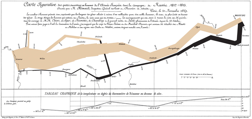
From Wikipedia;
“Étienne-Jules Marey first called notice to this dramatic depiction of the fate of Napoleon’s army in the Russian campaign, saying it defies the pen of the historian in its brutal eloquence. Edward Tufte says it “may well be the best statistical graphic ever drawn” and uses it as a prime example in The Visual Display of Quantitative Information.”
Wikipedia has a great explanation of the diagram type and there is a wealth of information dedicated to it on the inter-web. I heartily recommend http://www.sankey-diagrams.com/ for all things Sankey!
So it would come as little surprise that Mike Bostock has developed a plugin for Sankey diagrams (http://bost.ocks.org/mike/sankey/) so that we can all enjoy Sankey goodness with lashings of D3.
Which Sankey plugin should we use?
Hmmmm…… Good question.
As at the time of writing there were 4 different sankey plugins listed on the d3 wiki (including the vertical one). The examples we will walk through have used the plugins from Stefaan Lippens and Jason Davies without problem. I have used the Jason Davies version for no other reason than it appears to be the originator from which others have been derived.
How d3.js Sankey Diagrams want their data formatted
If we think of Sankey diagrams consisting of ‘nodes’ and ‘links’…
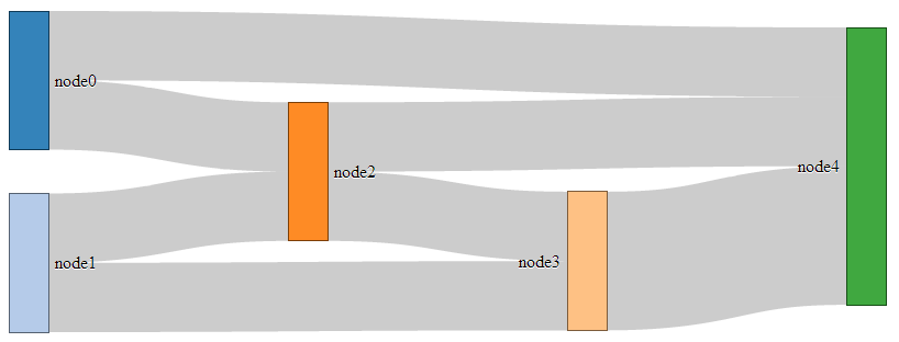
… the data that generates them must be formatted as nodes and links as well.
For instance a JSON file with appropriate data to build the diagram above could look like the following;
In the file above we have 6 nodes (0-5) sequentially numbered and with names appropriate to their position in the list.
The sequential numbering is only for the purpose of highlighting the structure of the data, since when we get D3 running, it will automatically index each of the nodes according to its position. In other words, we could have omitted the “node”:n parts since D3 will know where each node is anyway. The big deal is that WE need to know what each node is as well. Especially if we’re going to be building the data by hand (doing it dynamically would be cool, but let’s not get ahead of ourselves just yet).
The ‘links’ part of the data can be broken down into individual source to target ‘links’ that have an associated value (could be a quantity or strength, but at least a numeric value).
The ‘source’ and ‘target’ numbers are references to the list of nodes. So, “source”:1, “target”:2 means that this link is whatever node appears at position 1 going to whatever node appears at position 2. The important point to make here is that D3 will not be interested in the numerical value of the node, just its position in the list (starting at zero).
Description of the code
The code for the Sankey diagram is significantly different to that for a line graph although it shares the same core language and programming methodology.
The code we’ll go through is an adaptation of the version first demonstrated by Mike Bostock so it’s got a pretty good pedigree. We will begin with a version that uses data that is formatted so that it can be used directly with no manipulation, then in subsequent sections we will work on different techniques for getting data from different formats (and with different structures) to work.
I found that getting data in the correct format was the biggest hurdle for getting a Sankey diagram to work. We will start off assuming that the data is perfectly formatted, then where only the link data is available, then where there is just names to work with (no numeric node values) and lastly, one that can be used for people with changeable data from a MySQL database.
We won’t try to go over every inch of the code as we did with the simple graph example (I’ll skip things like the HTML header) and will focus on the style sheet (CSS) portion and the JavaScript.
The full code for this example can be found on github or in the code samples bundled with this book (sankey-formatted-json.html, sankey.js and sankey.json). A live example can be found on bl.ocks.org.
On to the code…
<!DOCTYPE html>
<meta charset="utf-8">
<title>SANKEY Experiment</title>
<style>
.node rect {
cursor: move;
fill-opacity: .9;
shape-rendering: crispEdges;
}
.node text {
pointer-events: none;
text-shadow: 0 1px 0 #fff;
}
.link {
fill: none;
stroke: #000;
stroke-opacity: .2;
}
.link:hover {
stroke-opacity: .5;
}
</style>
<body>
<script src="https://d3js.org/d3.v4.min.js"></script>
<script src="sankey.js"></script>
<script>
var units = "Widgets";
// set the dimensions and margins of the graph
var margin = {top: 10, right: 10, bottom: 10, left: 10},
width = 700 - margin.left - margin.right,
height = 300 - margin.top - margin.bottom;
// format variables
var formatNumber = d3.format(",.0f"), // zero decimal places
format = function(d) { return formatNumber(d) + " " + units; },
color = d3.scaleOrdinal(d3.schemeCategory20);
// append the svg object to the body of the page
var svg = d3.select("body").append("svg")
.attr("width", width + margin.left + margin.right)
.attr("height", height + margin.top + margin.bottom)
.append("g")
.attr("transform",
"translate(" + margin.left + "," + margin.top + ")");
// Set the sankey diagram properties
var sankey = d3.sankey()
.nodeWidth(36)
.nodePadding(40)
.size([width, height]);
var path = sankey.link();
// load the data
d3.json("sankey.json", function(error, graph) {
sankey
.nodes(graph.nodes)
.links(graph.links)
.layout(32);
// add in the links
var link = svg.append("g").selectAll(".link")
.data(graph.links)
.enter().append("path")
.attr("class", "link")
.attr("d", path)
.style("stroke-width", function(d) { return Math.max(1, d.dy); })
.sort(function(a, b) { return b.dy - a.dy; });
// add the link titles
link.append("title")
.text(function(d) {
return d.source.name + " → " +
d.target.name + "\n" + format(d.value); });
// add in the nodes
var node = svg.append("g").selectAll(".node")
.data(graph.nodes)
.enter().append("g")
.attr("class", "node")
.attr("transform", function(d) {
return "translate(" + d.x + "," + d.y + ")"; })
.call(d3.drag()
.subject(function(d) {
return d;
})
.on("start", function() {
this.parentNode.appendChild(this);
})
.on("drag", dragmove));
// add the rectangles for the nodes
node.append("rect")
.attr("height", function(d) { return d.dy; })
.attr("width", sankey.nodeWidth())
.style("fill", function(d) {
return d.color = color(d.name.replace(/ .*/, "")); })
.style("stroke", function(d) {
return d3.rgb(d.color).darker(2); })
.append("title")
.text(function(d) {
return d.name + "\n" + format(d.value); });
// add in the title for the nodes
node.append("text")
.attr("x", -6)
.attr("y", function(d) { return d.dy / 2; })
.attr("dy", ".35em")
.attr("text-anchor", "end")
.attr("transform", null)
.text(function(d) { return d.name; })
.filter(function(d) { return d.x < width / 2; })
.attr("x", 6 + sankey.nodeWidth())
.attr("text-anchor", "start");
// the function for moving the nodes
function dragmove(d) {
d3.select(this)
.attr("transform",
"translate("
+ d.x + ","
+ (d.y = Math.max(
0, Math.min(height - d.dy, d3.event.y))
) + ")");
sankey.relayout();
link.attr("d", path);
}
});
</script>
</body>
So, going straight to the style sheet bounded by the <style> tags;
.node rect {
cursor: move;
fill-opacity: .9;
shape-rendering: crispEdges;
}
.node text {
pointer-events: none;
text-shadow: 0 1px 0 #fff;
}
.link {
fill: none;
stroke: #000;
stroke-opacity: .2;
}
.link:hover {
stroke-opacity: .5;
}
The CSS in this example is mainly concerned with formatting of the mouse cursor as it moves around the diagram.
The first part…
.node rect {
cursor: move;
fill-opacity: .9;
shape-rendering: crispEdges;
}
… provides the properties for the node rectangles. It changes the icon for the cursor when it moves over the rectangle to one that looks like it will move the rectangle (there is a range of different icons that can be defined here http://www.echoecho.com/csscursors.htm), sets the fill colour to mostly opaque and keeps the edges sharp.
The next block…
.node text {
pointer-events: none;
text-shadow: 0 1px 0 #fff;
}
… sets the properties for the text at each node. The mouse is told to essentially ignore the text in favour of anything that’s under it (in the case of moving or highlighting something else) and a slight shadow is applied for readability).
The following block…
.link {
fill: none;
stroke: #000;
stroke-opacity: .2;
}
… makes sure that the link has no fill (it actually appears to be a bendy rectangle with very thick edges that make the element appear to be a solid block), colours the edges black (#000) and makes the edges almost transparent.
The last block….
.link:hover {
stroke-opacity: .5;
}
… simply changes the opacity of the link when the mouse goes over it so that it’s more visible. If so desired, we could change the colour of the highlighted link by adding in a line to this block changing the colour like this stroke: red;.
Just before we get into the JavaScript, we do something a little different for d3.js. We tells it to use a plug-in with the following line;
<script src="sankey.js"></script>
The concept of a plug-in is that it is a separate piece of code that will allow additional functionality to a core block (which in this case is d3.js). There are a range of plug-ins available and we will need to source the sankey.js file from the repository and place that somewhere where our HTML code can access it. In this case I have put it in the same directory as the main sankey web page.
The start of our JavaScript begins by defining a range of variables that we’ll be using.
Our units are set as ‘Widgets’ (var units = "Widgets";), which is just a convenient generic (nonsense) term to provide the impression that the flow of items in this case is widgets being passed from one person to another.
We then set our canvas size and margins…
var margin = {top: 10, right: 10, bottom: 10, left: 10},
width = 700 - margin.left – margin.right,
height = 300 - margin.top – margin.bottom;
… before setting some formatting.
var formatNumber = d3.format(",.0f"), // zero decimal places
format = function(d) { return formatNumber(d) + " " + units; },
color = d3.scaleOrdinal(d3.schemeCategory20);
The formatNumber function acts on a number to set it to zero decimal places in this case. In the original Mike Bostock example it was to three places, but for ‘widgets’ I’m presuming we don’t divide :-).
format is a function that returns a given number formatted with formatNumber as well as a space and our units of choice (‘Widgets’). This is used to display the values for the links and nodes later in the script.
The color = d3.scaleOrdinal(d3.schemeCategory20); line is really interesting and provides access to a colour scale that is pre-defined for your convenience! Later in the code we will see it in action.
Our next block of code positions our svg element onto our page in relation to the size and margins we have already defined;
var svg = d3.select("body").append("svg")
.attr("width", width + margin.left + margin.right)
.attr("height", height + margin.top + margin.bottom)
.append("g")
.attr("transform",
"translate(" + margin.left + "," + margin.top + ")");
Then we set the variables for our sankey diagram;
var sankey = d3.sankey()
.nodeWidth(36)
.nodePadding(40)
.size([width, height]);
Without trying to state the obvious, this sets the width of the nodes (.nodeWidth(36)), the padding between the nodes (.nodePadding(40)) and the size of the diagram(.size([width, height]);).
The following line defines the path variable as a pointer to the sankey function that makes the links between the nodes do their clever thing of bending into the right places;
var path = sankey.link();
I make the presumption that this is a defined function within sankey.js.
Then we load the data for our sankey diagram with the following line;
d3.json("sankey.json", function(error, graph) {
As we have seen in previous usage of the d3.json, d3.csv and d3.tsv functions, this is a wrapper that acts on all the code within it bringing the data in the form of graph to the remaining code.
I think it’s a good time to take a slightly closer look at the data that we’ll be using;
I want to look at the data now, because it highlights how it is accessed throughout this portion of the code. It is split into two different blocks, ‘nodes’ and ‘links’. The subset of variables available under ‘nodes’ is ‘node’ and ‘name’. Likewise under ‘links’ we have ‘source’, ‘target’ and ‘value’. This means that when we want to act on a subset of our data we define which piece by defining the hierarchy that leads to it. For instance, if we want to define an action for all the links, we would use graph.links (they’re kind of chained together).
Now that we have our data loaded, we can assign the data to the sankey function so that it knows how to deal with it behind the scenes;
sankey
.nodes(graph.nodes)
.links(graph.links)
.layout(32);
In keeping with our previous description of what’s going on with the data, we have told the sankey function that the nodes it will be dealing with are in graph.nodes of our data structure.
I’m not sure what the .layout(32); portion of the code does, but I’d be interested to hear from any more knowledgeable readers. I’ve tried changing the values to no apparent effect and googling has drawn a blank. Internally to the sankey.js file it seems to indicate ‘iterations’ while it establishes computeNodeLinks, computeNodeValues, computeNodeBreadths, computeNodeDepths (iterations) and computeLinkDepths.
Then we add our links to the diagram with the following block of code;
var link = svg.append("g").selectAll(".link")
.data(graph.links)
.enter().append("path")
.attr("class", "link")
.attr("d", path)
.style("stroke-width", function(d) { return Math.max(1, d.dy); })
.sort(function(a, b) { return b.dy - a.dy; });
This is an analogue of the block of code we examined way back in the section that we covered in explaining the code of our first simple graph.
We append svg elements for our links based on the data in graph.links, then add in the paths (using the appropriate CSS). We set the stroke width to the width of the value associated with each link or ‘1’. Whichever is the larger (by virtue of the Math.max function). As an interesting sideline, if we force this value to ‘10’ thusly…
.style("stroke-width", 10)
… the graph looks quite interesting.
The sort function (.sort(function(a, b) { return b.dy - a.dy; });) makes sure the link for which the target has the highest y coordinate departs first out of the rectangle. Meaning if you have flows of 30,40,50 out of node 1, heading towards nodes 2, 3 and 4, with node 3 located above node 2 and that above node 4, the outflow order from node 1 will be 40,50,30. This makes sure there are a minimum of flow crosses. It’s slightly confusing and for a long time it was a mystery (big thanks and kudos to ‘napicool’ who was able to explain it on d3noob.org.
The next block adds the titles to the links;
link.append("title")
.text(function(d) {
return d.source.name + " → " +
d.target.name + "\n" + format(d.value); });
This code appends a text element to each link when moused over that contains the source and target name (with a neat little arrow in between and the value) which, when applied with the format function, adds the units.
The next block appends the node objects (but not the rectangles or text) and contains the instructions to allow them to be arranged with the mouse.
var node = svg.append("g").selectAll(".node")
.data(graph.nodes)
.enter().append("g")
.attr("class", "node")
.attr("transform", function(d) {
return "translate(" + d.x + "," + d.y + ")"; })
.call(d3.drag()
.subject(function(d) {
return d;
})
.on("start", function() {
this.parentNode.appendChild(this);
})
.on("drag", dragmove));
While it starts off in familiar territory with appending the node objects using the graph.nodes data and putting them in the appropriate place with the transform attribute, I can only assume that there is some trickery going on behind the scenes to make sure the mouse can do what it needs to do with the d3.behaviour,drag function. There is some excellent documentation on the wiki, but I can only presume that it knows what it’s doing :-). The dragmove function is laid out at the end of the code, and we will explain how that operates later. Kudos for this code portion should go to @syntagmatic.
I really enjoyed the next block;
node.append("rect")
.attr("height", function(d) { return d.dy; })
.attr("width", sankey.nodeWidth())
.style("fill", function(d) {
return d.color = color(d.name.replace(/ .*/, "")); })
.style("stroke", function(d) {
return d3.rgb(d.color).darker(2); })
.append("title")
.text(function(d) {
return d.name + "\n" + format(d.value); });
It starts off with a fairly standard appending of a rectangle with a height generated by its value { return d.dy; } and a width dictated by the sankey.js file to fit the area (.attr("width", sankey.nodeWidth())).
Then it gets interesting.
The colours are assigned in accordance with our earlier colour declaration and the individual colours are added to the nodes by finding the first part of the name for each node and assigning it a colour from the palate (the script looks for the first space in the name using a regular expression). For instance: ‘Widget X’, ‘Widget Y’ and ‘Widget’ will all be coloured the same even if the ‘Widget X’ and ‘Widget Y’ are inputs on the left and ‘Widget’ is a node in the middle.
The stroke around the outside of the rectangle is then drawn in the same shade, but darker.
Then we return to the basics where we add the title of the node in a tool tip type effect along with the value for the node.
From here we add the titles for the nodes;
node.append("text")
.attr("x", -6)
.attr("y", function(d) { return d.dy / 2; })
.attr("dy", ".35em")
.attr("text-anchor", "end")
.attr("transform", null)
.text(function(d) { return d.name; })
.filter(function(d) { return d.x < width / 2; })
.attr("x", 6 + sankey.nodeWidth())
.attr("text-anchor", "start");
Again, this looks pretty familiar. We position the text titles carefully to the left of the nodes. All except for those affected by the filter function (return d.x < width / 2;). Where if the position of the node on the x axis is less than half the width, the title is placed on the right of the node and anchored at the start of the text. Very neat.
The last block is also pretty neat, and contains a little surprise for those who are so inclined.
function dragmove(d) {
d3.select(this)
.attr("transform",
"translate("
+ d.x + ","
+ (d.y = Math.max(
0, Math.min(height - d.dy, d3.event.y))
) + ")");
sankey.relayout();
link.attr("d", path);
This declares the function that controls the movement of the nodes with the mouse.
It selects the item that it’s operating over (d3.select(this)) and then allows translation in the y axis while maintaining the link connection (sankey.relayout(); link.attr("d", path);).
But that’s not the cool part. A quick look at the code should reveal that if you can move a node in the y axis, there should be no reason why you can’t move it in the x axis as well!
Sure enough, if you replace the code above with this…
function dragmove(d) {
d3.select(this).attr("transform",
"translate(" + (
d.x = Math.max(0, Math.min(width - d.dx, d3.event.x))
)
+ "," + (
d.y = Math.max(0, Math.min(height - d.dy, d3.event.y))
) + ")");
sankey.relayout();
link.attr("d", path);
… you can move your nodes anywhere on the canvas.
I know it doesn’t seem to add anything to the diagram (in fact, it could be argued that there is a certain aspect of detraction) however, it doesn’t mean that one day the idea doesn’t come in handy :-). You can see a live version on bl.ocks.org.
Formatting data for Sankey diagrams
From a JSON file with numeric link values
As explained in the previous section, data to form a Sankey diagram needs to be a combination of nodes and links.
{
"nodes":[
{"node":0,"name":"node0"},
{"node":1,"name":"node1"},
{"node":2,"name":"node2"},
{"node":3,"name":"node3"},
{"node":4,"name":"node4"}
],
"links":[
{"source":0,"target":2,"value":2},
{"source":1,"target":2,"value":2},
{"source":1,"target":3,"value":2},
{"source":0,"target":4,"value":2},
{"source":2,"target":3,"value":2},
{"source":2,"target":4,"value":2},
{"source":3,"target":4,"value":4}
]}
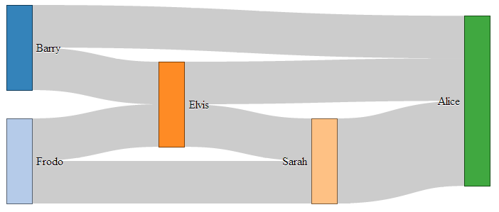
As we also noted earlier, the "node" entries in the "nodes" section of the JSON file are superfluous and are really only there for our benefit since D3 will automatically index the nodes starting at zero. As a test to check this out we can change our data to the following;
{
"nodes":[
{"name":"Barry"},
{"name":"Frodo"},
{"name":"Elvis"},
{"name":"Sarah"},
{"name":"Alice"}
],
"links":[
{"source":0,"target":2,"value":2},
{"source":1,"target":2,"value":2},
{"source":1,"target":3,"value":2},
{"source":0,"target":4,"value":2},
{"source":2,"target":3,"value":2},
{"source":2,"target":4,"value":2},
{"source":3,"target":4,"value":4}
]}
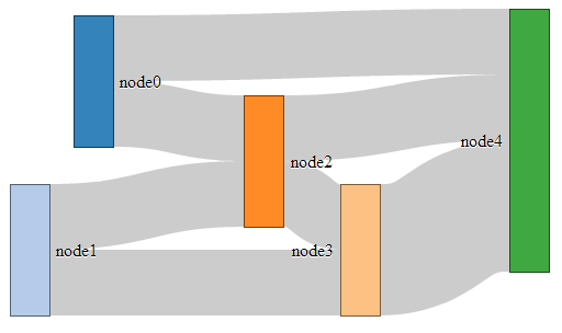
This will produce the following graph;

As you can see, essentially the same, but with easier to understand names.
As you can imagine, while the end result is great, the creation of the JSON file manually would be painful at best. Doing something similar but with a greater number of nodes / links would be a nightmare.
Let’s see if we can make the process a bit easier and more flexible.
From a JSON file with links as names
It would make thing much easier, if you are building the data from hand, to have nodes with names, and the ‘source’ and ‘target’ links to have those same name values as identifiers.
In other words a list of unique names for the nodes (and perhaps some details) and a list of the links between those nodes using the names for the nodes.
So, something like this;
{
"nodes":[
{"name":"Barry"},
{"name":"Frodo"},
{"name":"Elvis"},
{"name":"Sarah"},
{"name":"Alice"}
],
"links":[
{"source":"Barry","target":"Elvis","value":2},
{"source":"Frodo","target":"Elvis","value":2},
{"source":"Frodo","target":"Sarah","value":2},
{"source":"Barry","target":"Alice","value":2},
{"source":"Elvis","target":"Sarah","value":2},
{"source":"Elvis","target":"Alice","value":2},
{"source":"Sarah","target":"Alice","value":4}
]}
Once again, D3 to the rescue!
The little piece of code that can do this for us is here;
var nodeMap = {};
graph.nodes.forEach(function(x) { nodeMap[x.name] = x; });
graph.links = graph.links.map(function(x) {
return {
source: nodeMap[x.source],
target: nodeMap[x.target],
value: x.value
};
});
This elegant solution comes from Stack Overflow and was provided by Chris Pettitt (nice job).
So if we sneak this piece of code into here…
d3.json("sankey-names.json", function(error, graph) {
// <= Put the code here.
  sankey
      .nodes(graph.nodes)
      .links(graph.links)
      .layout(32);
… and this time we use our JSON file with just names (sankey-names.json) and our new html file (sankey-formatted-names.html) we find our Sankey diagram working perfectly!
The full code for this example can be found on github or in the code samples bundled with this book (sankey-formatted-names.html, sankey.js and sankey-names.json). A live example can be found on bl.ocks.org.
Looking at our new piece of code…
    var nodeMap = {};
    graph.nodes.forEach(function(x) { nodeMap[x.name] = x; });
… the first thing it does is create an object called nodeMap (The difference between an array and an object in JavaScript is one that is still a little blurry to me and judging from online comments, I am not alone).
Then for each of the graph.node instances (where x is a range of numbers from 0 to the last node), we assign each node name to a number.
Then in the next piece of code…
    graph.links = graph.links.map(function(x) {
      return {
        source: nodeMap[x.source],
        target: nodeMap[x.target],
        value: x.value
      };
… we go through all the links we have and for each link, we map the appropriate number to the correct name.
Very clever.
From a CSV with ‘source’, ‘target’ and ‘value’ info only.
In the first iteration of this section of the book I had no solution to creating a Sankey diagram using a csv file as the source of the data.
But cometh the hour, cometh the man. Enter @timelyportfolio who, while claiming no expertise in D3 or JavaScript was able to demonstrate a solution to exactly the problem I was facing! Well done Sir! I salute you and name the technique the timelyportfolio csv method!
The full code for this example can be found on github or in the code samples bundled with this book (sankey-formatted-csv.html, sankey.js and sankey.csv). A live example can be found on bl.ocks.org.
So here’s the cleverness that @timelyportfolio demonstrated;
Using a csv file (in this case called sankey.csv) that looks like this;
We take this single line from our original Sankey diagram code;
d3.json("sankey-formatted.json", function(error, graph) {
And replace it with the following block;
d3.csv("sankey.csv", function(error, data) {

  //set up graph in same style as original example but empty
  graph = {"nodes" : [], "links" : []};

  data.forEach(function (d) {
    graph.nodes.push({ "name": d.source });
    graph.nodes.push({ "name": d.target });
    graph.links.push({ "source": d.source,
                       "target": d.target,
                       "value": +d.value });
   });

  // return only the distinct / unique nodes
  graph.nodes = d3.keys(d3.nest()
    .key(function (d) { return d.name; })
    .object(graph.nodes));

  // loop through each link replacing the text with its index from node
  graph.links.forEach(function (d, i) {
    graph.links[i].source = graph.nodes.indexOf(graph.links[i].source);
    graph.links[i].target = graph.nodes.indexOf(graph.links[i].target);
  });

  // now loop through each nodes to make nodes an array of objects
  // rather than an array of strings
  graph.nodes.forEach(function (d, i) {
    graph.nodes[i] = { "name": d };
  });
The comments in the code (and they are fuller in @timelyportfolio’s original gist solution) explain the operation;
d3.csv("sankey.csv", function(error, data) {
… Loads the csv file from the data directory.
graph = {"nodes" : [], "links" : []};
… Declares graph to consist of two empty arrays called nodes and links.
      data.forEach(function (d) {
      graph.nodes.push({ "name": d.source });
      graph.nodes.push({ "name": d.target });
      graph.links.push({ "source": d.source,
                         "target": d.target,
                         "value": +d.value });
     });
… Takes the data loaded with the csv file and for each row loads variables for the source and target into the nodes array. Then for each row it loads variables for the source target and value into the links array.
     graph.nodes = d3.keys(d3.nest()
       .key(function (d) { return d.name; })
       .object(graph.nodes));
… Is a routine that Mike Bostock described on Google Groups that (as I understand it) nests each node name as a key so that it returns with only unique nodes.
     graph.links.forEach(function (d, i) {
       graph.links[i].source = graph.nodes.indexOf(graph.links[i].source);
       graph.links[i].target = graph.nodes.indexOf(graph.links[i].target);
     });
… Goes through each link entry and, for each source and target, it finds the unique index number of that name in the nodes array and assigns the link source and target an appropriate number.
And finally…
     graph.nodes.forEach(function (d, i) {
       graph.nodes[i] = { "name": d };
     });
… Goes through each node and (in the words of @timelyportfolio) “make nodes an array of objects rather than an array of strings” (I don’t really know what that means :-(. I just know it works :-).)
There you have it. A Sankey diagram from a csv file. Well played @timelyportfolio!