Chapter 2 - Genomic Data Science With Galaxy
I never dreamed that in my lifetime my own genome would be sequenced.
James D. Watson
Why use Galaxy?
- Galaxy has grown out of several developments in genomics and data science. First, the scientific community realizes that reproducible work and work flows are extremely important to capture completely. Secondly, reproducible research should increase accessibility. Reproducibility, as it is now called, has several aims.
Reproducible Research aims to:
- Provide original data or clearly list its source,
- Provide cleaned data and a list of steps used to clean that data,
- Provide all code used or steps taken to process the cleaned data into tables, graphics, etc.,
- Reproducibility is the ability of an entire analysis of an experiment or study to be duplicated or replicated if so desired,
- Overall, reproducibility MEANS scientific work should be described in sufficient detail such that it can be precisely reproduced by another person in another environment.
But, what does Galaxy do?
- Galaxy has Genomics Analysis Tools for:
- Genomic assembly, RNA-Seq, or simple FASTA manipulation.
- Create Uniform Pipelines & tracks details
- Galaxy provides Workflow systems for replication, sharing of work
- Galaxy provides a platform for visualization
- Galaxy can facilitate communication, teaching/learning & even publishing
Galaxy is IMPORTANLY an extensible platform for sharing data and workflows. Galaxy can be run on public or private servers but it is easy to install it and run it locally on a laptop.
2.1 - First Steps: Register with Galaxy
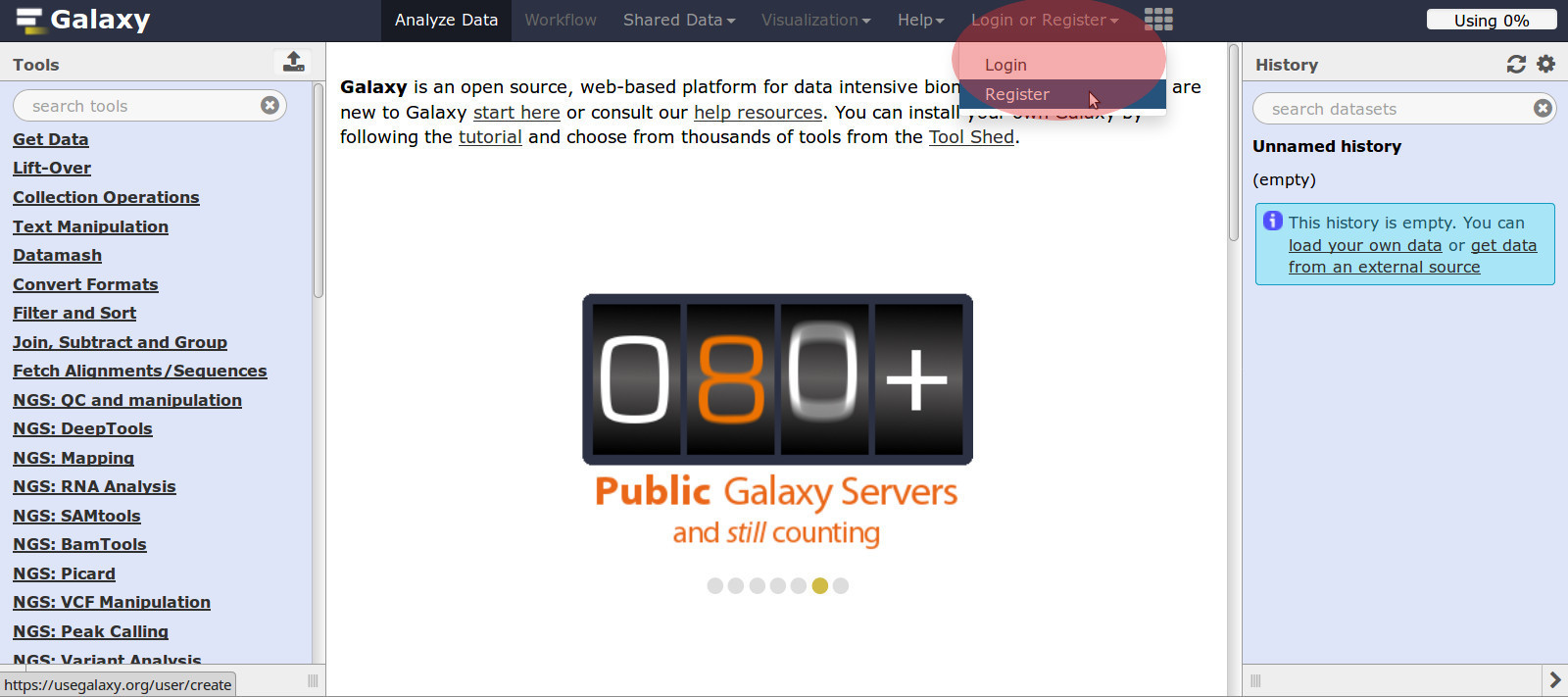
2.1.1 - Register A New Account at (https://usegalaxy.org)
- Open the UseGalaxy web page.
- Go to the top middle section, in the red circle above.
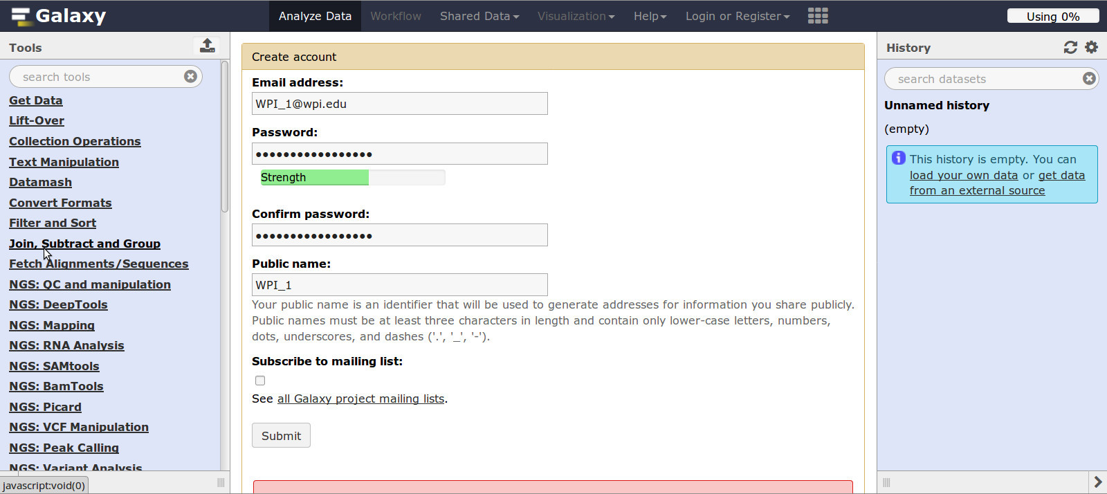
- Click: Login or Register / Register / Create account
- Fill in all account information
- Submit
2.1.2 - Explore Galaxy
The main Galaxy web page has 4 sections.
Galaxy top banner:

- Go to: Help
- Explore: Videos, Interactive Tours, Ask a question, …
- Watch: Introduction to Galaxy by James Taylor, PhD, Assoc. Professor at Johns Hopkins Uni.
Tools (on left):
- Here you can Get Data, Manipulate data, Sort and Fetch Alignments, and use NGS (Next Generation Sequencing) tools, etc.
- For example, choose a category, then choose an algorithm.
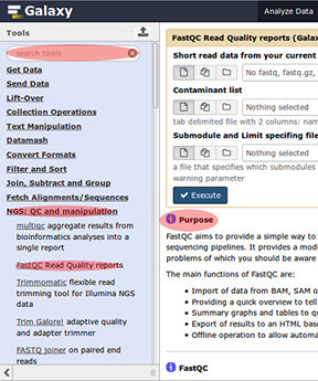
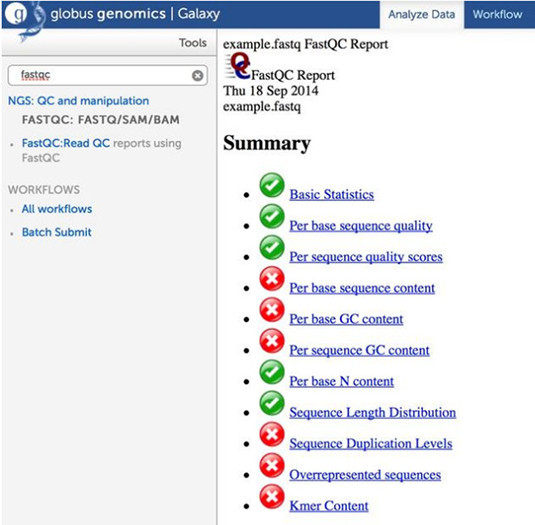
- Search for FastQC: either in the search bar or under NGS: QC and manipulation
Center panel:
The Center panel allows one to inspect data, results, generate step-wise workflows, visualize results, share and publish data.
- Now, Go to the Tools section
- Search: fastqc in the search tools oval and click FastQC
OR - Find: NGS: QC and manipulation and click FastQC
- Notice the help information showing what FASTQC does and how to operate it.
- In the Center Panel, READ the FASTQC help section, you will need this later.
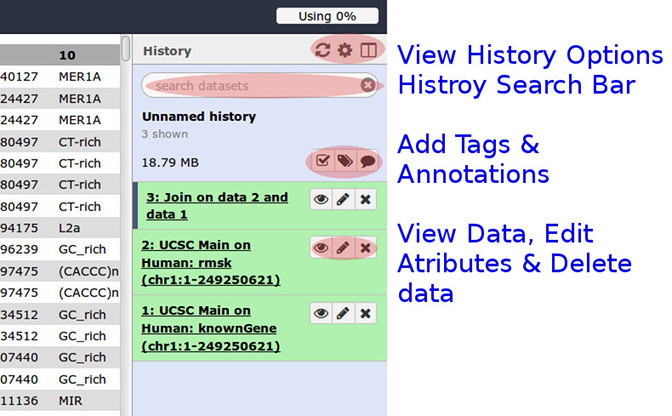
History (on right):
- History allows one to search and look over their past work, &
- Operate on multiple datasets, Edit History tags, & Add/Edit annotataions, also
- Once you start producing work files you may, View data, Edit attributes, or Delete your work.
Want more Information?
TRY THESE Video Tutorials, they are great!
But you can also find other Galaxy Tutorials Here.
2.2 - Exercise # 1: Investigating SNP on a chromosome
Q. Which coding exon has the highest number of single nucleotide polymorphisms on chromosome 22?
See paper: A map of human genome sequence variation containing 1.42 million single nucleotide polymorphisms, Nature 409, 928-933, 15 February 2001, The International SNP Map Working Group
Generalized Steps:
- Load human chromosome data from UCSC Table Browser
- Load human snp data
- Join the genomic datasets
- Identify and count which exons which have repeats
- Save, download, and report data
Specific Steps:
A. Load human chromosome dataset from UCSC Table Browser
- Log in to Galaxy
- Go to: Tools / Get Data
- In the list, Find & click: UCSC Main Table Browser
- download data from the Genome Table Browser database
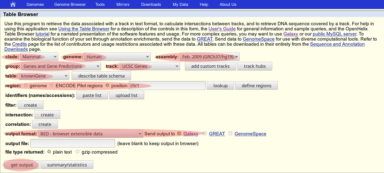
In Genome Table Browser choose/set:
- clade: Mammal
- genome: Human
- assembly: Feb 2009 (…/hg19)
- group: Genes and Gene Predictions
- track: UCSC Genes
- table: knownGene
- Click Radio button: position, type chr22
- output format: Set to BED
- Click Radio button: Send output to Galaxy
NOTE: Do not change other menu items.
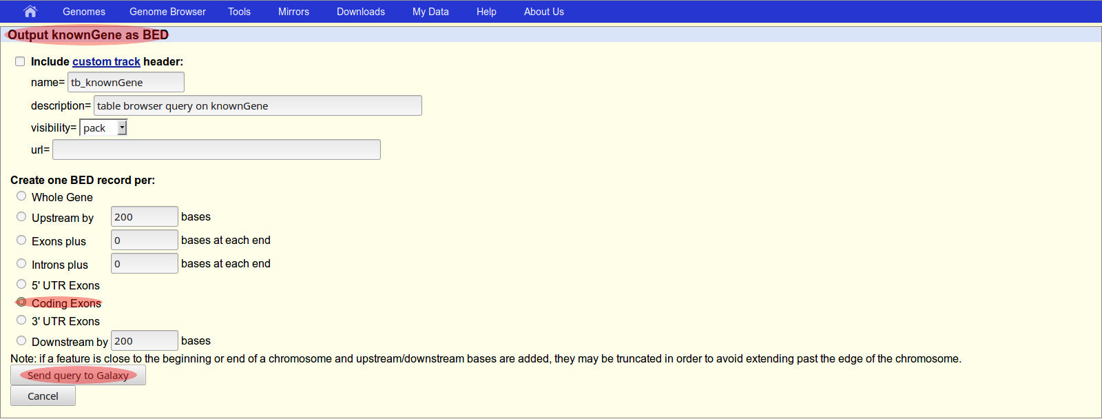
- A second screen entitled “Output knownGene as BED” will be shown next.
- On the Screen/Page #2: Output knownGene as BED file format
- Find: Create one BED record per:
- Click Radio button: Coding Exons
- Goto bottom button: Send query to Galaxy
- Note: This should return you to the Galaxy web page.
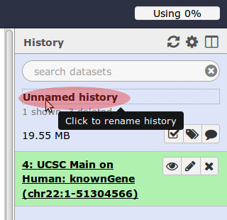
- You may rename your current ‘job’ from Unnamed history to chr snp codons
B. Download human snp data
Load Second Dataset, Repeats data:
- Go to: Tools / Get Data
- In the list, find & click: UCSC Main Table Browser
- download data from the Genome Table Browser database
In Genome Table Browser choose/set:
- clade: Mammal
- genome: Human
- assembly: Feb 2009 (…/hg19)
- group: Repeats
- track: RepeatMasker
- Click Radio button: position / Type: chr22
- output format: BED
- Send output to Galaxy
- Go to bottom button: get output
- On the Screen/Page #2: Output rmsk as BED
- Create one BED record per: Whole Gene
- Goto bottom button: Send query to Galaxy
Go to your History
- History should now show two datasets
- Click: the View data (EYE icon) and inspect datasets
- This is a BED file format file format.
- You may click: the Edit Attributes (PENCIL icon) to add any information or annotations to your data.
C. Join the genomic datasets
The Goal of this section is to perform an INNER JOIN on the datasets.

- Go to: Tools
- Search for: Operate on Genomic Intervals / Join
- In the center panel with the header: Join
- Join, First dataset: Set - UCSC Human knownGene
- with, Second dataset: Set - UCSC Human rmsk
- Go to: with min overlap Set - 1 bp
- Go to: Return Set - Only records that are joined (INNER JOIN)
- Execute
- See the aside box above: Look in the History panel …
D. Identify & count the overlaps from the joined dataset
The Goal of this section is to identify which exons have repeats.
- Once Inner Join is finished
- Go to: Tools
- Go to: Join, Subtract and Grouping
- Go to: Group
- The Group data tool will appear in center panel.
- Select data: Joined dataset
- Group by Column: Set - Column 4
- Go to bottom: Operation Click: + Insert Operation
- Type: Count – Note: We want the count of all overlaps.
- On column: Column 4
- Click: Execute
- Once Count is finished
- Go to: History & View data (Click Eye icon)
Q. What are these two columns What do they represent?
- This data shows the exon name and count next in the middle panel.
- We have answered our question, but we can do better.
Check below
E. Incorporate (Join) the overlap counts with the Exon information
- Return to: Tools
- Go to: Join, Subtract, and Group
- Go to: Join two Datasets…
- In the middle panel, choose the known genes from first dataset.
- Set - Using column: Column 4
- With: Inner joined dataset
- Set - and column: Column 1
- Execute
- Once the join is complete we can view the results,
- Go to: History
- Go to: View data
- Go to: Tools
- Go to: Text Manipulation
- Go to: Cut
- Cut columns: c1, c2, c3, c4, c8
- Execute
- Note: You may save this final file to your computer:
- Click: History / Cut on data 5 / “floppy disk icon”
- Report findings
- Stop Here
2.3 - Exercise # 2: FASTA & FASTQ file formats
?Describe NGS?
Q. What are FASTA & FASTQ file formats? Explain?
The first two file formats which will be discussed are FASTA and FASTQ files. Sometimes using the file extensions .fasta, .fa, .fastq, ???
The FASTA format:
1 \>ACCESSION   AAD28535.1
2 MEEPQSDPSVEPPLSQETFSDLWKLLPENNVLSPLPSQAMDDLMLSPDDIEQWFTEDPGPDEAPRMPEAA
3 PRVAPAPAAPTPAAPAPAPSWPLSSSVPSQKTYQGSYGFRLGFLHSGTAKSVTCTYSPALNKMFCQLAKT
4 CPVQLWVDSTPPPGTRVRAMAIYKQSQHMTEVVRRCPHHERCSDSDGLAPPQHLIRVEGNLRVEYLDDRN
5 TFRHSVVVPYEPPEVGSDCTTIHYNYMCNSSCMGGMNRRPILTIITLEDSSGNLLGRNSFEVRVCACPGR
6 DRRTEKENLRKKGEPHHELPPGSTKRALPNNTSSSPQPKKKPLDGEYFTLQIRGRERFEMFRELNEALEL
7 KDAQAGKEPGGSRAHSSHLKSKKGQSTSRHKKLMFKTEGPDSD
The FASTQ format:
1 @SEQ_ID
2 GATTTGGGGTTCAAAGCAGTATCGATCAAATAGTAAATCCATTTGTTCAACTCACAGTTT
3 +
4 !''*((((***+))%%%++)(%%%%).1***-+*''))**55CCF>>>>>>CCCCCCC65
- Go to: Shared Data
- Data Libraries
- Illumina iDEA Datasets (sub-sampled)
- BT20 paired-end RNA-seq subsampled (end 1)
NGS Data Quality Control
- FASTQ format
- Examine quality in an Chip-Seq dataset
- Trim/filter as we see ft, hopefully without breaking anything.
Assessment tools
- NGS QC and Manipulation to FastQC
- https://en.wikipedia.org/wiki/FASTQ_format
- Gives you a lot of information but little control over how it is calculated or presented.
2.4.2 What is FASTQ?
- Specifies sequence (FASTA) and quality scores (PHRED)
- https://en.wikipedia.org/wiki/Phred_quality_score
- Text format, 4 lines per entry
FastQC - Assessment tools
-
NGS QC and Manipulation / FastQC
- Gives you a lot of information but little control over how it is calculated or presented.
- UpLoad your dataset to line Short read data from your current history
- Other options not necessary now
- Execute
- This produces an HTML report of the data in the History panel.
- Click on the View data (Eye icon) to view the report in the middle panel.
Base Quality Trimming - Option 1
- NGS: QC and Manipulation / FASTQ Trimmer by column
- Trim same number of columns from every record
- Can specify different trim for 5 prime and 3 prime ends
- NGS: QC and Manipulation / Trim sequences
- Place dataset in top box
- In second and third boxes, select which bases to keep from x to y.
- Execute
Base Quality Trimming - Option 2
- NGS QC and Manipulation -> Select high quality segments.
- Select by score & length
- Keep or discard whole reads
- Can have different thresholds for different regions of the reads.
- Keeps original read length.
Base Quality Trimming - Option 3
- Trim as we see fit: Option 3
- NGS QC and Manipulation -> Manipulate FASTQ
- By sliding ‘window’ one can fine tune reads
- e.g. Trim from both ends, using sliding windows, until you hit a high-quality section.
- Produces variable length reads
Trim? As we see fit? - Option 4
- NGS QC and Manipulation -> FASTQ Quality Trimmer by sliding window
- Choice depends on downstream tools
- Find out assumptions & requirements for downstream tools and make appropriate choice(s) now.
2.4 - Exercise # 3: ChIP-Seq analysis with MACS
Q. What is ChIP-Seq analysis with MACS? And what does it investigate?
A fast and powerful analysis algorithm, titled Model- based Analysis of Tiling-arrays (MAT), reliably detect[s] regions enriched by transcription factor chromatin immunoprecipitation (ChIP),
Model-based analysis of tiling-arrays for ChIP-chip, Proc Natl Acad Sci, U S A, 2006 Aug 15; 103(33): 12457–12462
See paper: Model-based analysis of ChIP-Seq (MACS), Genome Biol. 2008; 9, 9, Zhang Y et al
Generalized steps:
- Load Demonstration datasets
- Analyze Data
- Find Peaks
Specific steps:
A. Load Demonstration datasets
- Go to History: Create New History
- Rename History to: Mouse - MACS G1E_CTCF
- Go to Top bar: Shared Data
- Click: Data Libraries
- Click: Demonstration Datasets
- Description: Demonstration datasets collected from various Galaxy tutorials
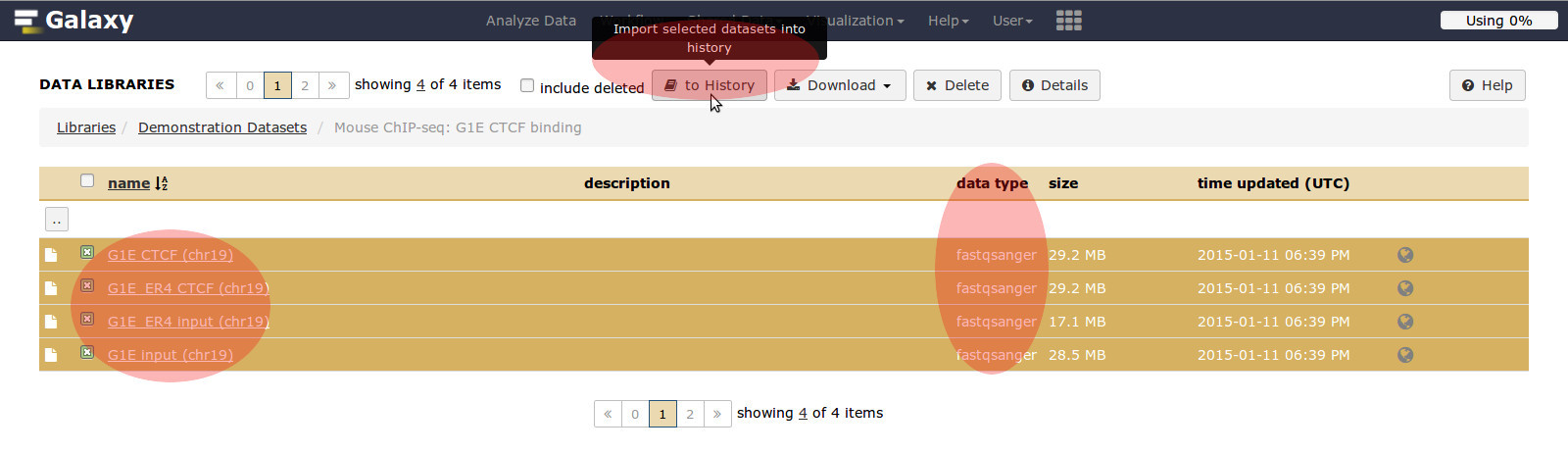
- Click Radio button: Mouse Chip-seq G1E CTCF binding
- Description: Sample datasets from Hardison lab for ChIP-seq analysis from Hardison lab
- Highlight link
- Choose all 4 mouse data sets
Q1. What type of datasets are these?
Hint: Biostars.org Question
- Go to: Import to current history
B. Analyze Data
- Once loaded,
- Goto: Analyze Data
- NO, DO CONTROL: Usually we would do FASTQC quality control, however for this example we will skip it.
- Go to: Tools
- Go to: NGS Mapping
- Bowtie2 aligned reads sorted BAM**
- Bowtie2 - maps reads against a reference genome
- Bowtie2 will show in middle panel
- This data is single-end reads
Q2. What does single ended reads refer to? What are the advantages of using single ended pairs.
Hint: Beginner’s Handbook to Next Generation Sequencing
- Choose FASTQ / G1E CTCF (chr19)
- Select reference genome / Mouse (mus musculus): mm9
- Write unaligned reads (in fastq format) to separate file(s): YES
- Group 1: No, just use defaults
- Group 2: Do you want to use presets?: Very fast end-to-end (–very-fast)
- Save the bowtie2 mapping statistics to the history: YES
- Execute: Run bowtie2
Q3. What is .bam file format?
Hint: Samtools
***
- Find summary stats in the History box, number of reads, % unpaired, % aligned exactly 1 time, % aligned >1 time…
C. FIND PEAKS
- Go to: **Tools
- Go to: NGS: Peak Calling
- Go to: MACS
- Go to Middle Panel:.
- Go to: Experiment Name:
- Mouse - MACS G1E_CTCF
- Tag File: Bowtie2 on data #: aligned sorted BAM
- Tag Size: 36
- Leave MFOLD: 32
- Check: Perform the new peak detection method (future dir): YES
- Execute
- This will produce two files:
- MACS on data 5 (peaks:bed)
- MACS on data 5 (html report)
- Click on View data (Eye icon) to get more information.
- Download from the html report data set:
1 Additional Files:
2
3 - MACS_in_Galaxy_model.pdf
4 - MACS_in_Galaxy_model.r
- Goto: UCSC Main Genome Browser
Running controls in very important; MACS peak detection
- After shift, slide windows of size 2d across genome,
- Model tag count for windows as a Poisson distribution, and calculate a p-value for each window,
- For the (lambda) parameter (~expected number of tags per window), estimate from sample or control if available,
- Estimates for local windows of size 1kb, 5kb, 10kb or the whole genome and uses the max,
- RERUN CHIP-Seq with Control:
- NGS Mapping: Bowtie2 on G1E_Input** File #4, Single-end
- NGS: Peak Calling -> MACS On the resulting mapped reads
- Execute
- Run MACS again: NGS: Peak Calling
- Title can be: MACS on G1E_CTCF with Control
- Select data file #5, .BAM file
- Click / Chip-Seq Control File / Choose Control; Bowtie2 on data #4, aligned reads in BAM format
- Change Tag size: 32 bp
- Check box:
- Perform the new peak detection method (future dir): YES
- Execute
- Analyze…
- Goto: UCSC Main Genome Browser
-
2.5.2 Biases on your experiment:
In this experiment, where is bias introduced?
- Chromatin accessibility affects fragmentation
- Amplification bias
- Repetitive regions
- Solution: Controls
- Input DNA (after fragmentation but before IP)
- Non-specific IP
Summary
- MACS is one tool, available in Galaxy, for analysis of ChIP-seq data.
- Controls are extremely important for accurately calling ChIP-seq peaks.
- As for most genomics problems, there are other tools that may be appropriate depending on the type of data, for example SICER for broad histone modifications.
2.5 - Exercise # 4: RNA-Seq
Q. RNA-Seq Differential Expression…
General Directions; RNA-Seq Exercise
- Create new history
- (cog) -> Create New
- Get data;
- From Shared Data -> Data Libraries
- Demonstration Datasets / Human RNA-seq: CHB ENCODE Exercise / Select All 5 Datasets in folder
- Import to current history
NOTE: We’re ignoring quality control in this example, HOWEVER, in practice this would be a good time for FASTQC
INSERT PICTURE FROM SLIDES; RNA-SEQ MAPPING, SLIDE 5
NOTE: This data can be analyzed in many different ways depending on goals of the experiment, what other data is available, etc.
INSERT PICTURE FROM SLIDES; RNA-SEQ MAPPING, SLIDE 7
2.6.2 Two Approaches
- USE: Align-then-assemble: potentially more sensitive, but requires a reference genome, confounded by structural variation
- de novo: likely to only capture highly expressed transcripts, but does not require a reference genome, robust to variation.
- Mapping will be done using Tophat
- Find Tophat: Tools / NGS: RNA-seq / Tophat for Illumina
- In RNA-Seq FASTQ file: Select first data set, C20-rep1
- Drop down menu for built-in genome, choose hg-19
- We have single ended data.
- Use default settings
- Execute
- We see 4 NEW datasets on the right in the History panel.
- Insertions.bed, deletions.bed, splice junctions.bed, and accepted_hits.bam
NOW, we have multiple datasets that we want to run using the same set steps.
- Goto: Find Tophat: Tools / NGS: RNA-seq / Tophat for Illumina
- INSTEAD of choosing one file at a time.
- Hover over the 3 buttons on the top left, and find Multiple datasets, use Shift-Click you can choose multiple data files to run.
- AGAIN, WE REPEAT THE LAST STEPS.
- Drop down menu for built-in genome, choose hg-19
- We have single-ended data.
- Use default settings
- Execute
- ALL datasets will run.
- We SHOULD see 12 NEW datasets on the right in the History panel.
- Insertions.bed, deletions.bed, splice junctions.bed, and accepted_hits.bam
- CONTINUE AS NEEDED…To 2.6.3 RNA-Seq Analysis: Assembly Quantitation & Differential Expression
RNA-Seq Analysis: Assembly Quantitation & Differential Expression
- Use: Cufflinks, Cuffmerge, Cuffdiff
- Assembling RNA-seq data after mapping to a reference genome
- Spliced alignment provides estimates of
- locations of exons and
- splice junctions
- Is this information enough to know what transcripts are present?
Assemble Transcripts w/ Cufflinks
- NGS: RNA-seq -> Cufflinks
- Use reference annotation as guide:
- Gene Annotations (chr19)
NOTE: Need to do this for each of the four Tophat accepted_hits
outputs separately — use “run tool in parallel across multiple datasets”
- We will be using Accepted_hits.bam
- Goto: NGS: RNA-seq / Cufflinks
- We need to do several preliminary things:
- Use Reference Annotation / Use Reference Annotation as guide
- Select data set 5, chromosome 19-annotations.gtf
- This is, this is a file that came from data library and contains the gene annotation information.
- INSTEAD of choosing one file at a time, we want to run multiple files.
- Hover over the 3 buttons on the top left, and find Multiple datasets, use Shift-Click you can choose ALL 4 data files to run.
- Use default settings for all other options
- Execute - ALL 4 datasets will run with Cufflinks.
- It will provide sets of transcripts which are assembled using the reference genome as a guide.
- Each Cufflinks job will generate a couple of different data sets.
- Gene expression will be produced ans can be used to quantify actual the expression levels.
- The file reports FPKM and tracking_id which uses the .gft files annotations.
So now the question becomes which genes are differentially expressed and are they significant?
- However, we have one slight problem, which is that we have multiple cuffinks files making the comparison more difficult.
- We can solve this problem by merging the files using Cuffmerge
- Goto: Tools / NGS: RNA-seg / Cuffmerge
- Cuffmerge allows one to select multiple .gft files to merge.
- Use: Additional GTF input files for as many files as you want to merge.
- **Use: Reference Annotation / Yes / (e.g.) Chr19-annotation.gtf
- Execute
- The transcripts will merge to ONE file.
- Click on Eye icon to view, exons, start and end of exons, names of genes, etc.
Use Cuffdiff
- Goto: Tools / NGS: RNA-seg / Cuffdiff
- Use: Transcripts / Cuffmerge
- Goto: **Condition / ** At least two
- In our case, we have CD20 cells vs H1hesc
- For each condition, we have two replicates.
- Add replicates from Tophat2 work
- We will use Default values for this experiment BUT it is a good idea to read over the options…
- Execute
- WHAT FILE TYPE IS THIS?
- WHAT COLUMNS ARE RELEVANT? VALUE1 AND VALUE2, Log2(fold_change), p-value, q-value, significant, etc.
2.6 - Exercise # 5: RNA-Seq of 3 family members
Q. Matt Curcio’s Galaxy Project
Genomic Data Science with Galaxy
Title: RNA-Seq - Peer-graded Assignment - Galaxy Course Project
Name: Matthew Curcio
Submitted: 10/23/2016
2.9.1 Instructions:
The zip file fastq_bundle.zip contains six fastq files. These files contain targeted re-sequencing data for a father, mother and daughter trio (identified as NA12877, NA12878, and NA12880 respectively). The data consists of raw reads from an Illumina MiSeq sequencer sequenced as paired ends (R1/R2) to 125bp in length.
| Data Set | Relation |
|---|---|
| Coriell-NA12877 (R1/R2) | Father |
| Coriell-NA12878 (R1/R2) | Mother |
| Coriell-NA12880 (R1/R2) | Daughter |
- Table#1: Targeted Re-sequencing Raw Data From Illumina MiSeq Sequencer
Create a Galaxy workflow to identify polymorphic sites in all three individuals. Your workflow will need to map the three sets of paired reads to the appropriate reference genome. You will then need to use a variant caller to identify sites that appear to have strong support for the presence of a polymorphism, and call the genotype at that site for each sample.
You should report your results in VCF (variant call format). You should only include sites where the chance of a false positive call is 1 in 10,000 or better according to the VCF qual field.
Using your resulting VCF determine 1) the number of single nucleotide variants, 2) the number of insertion/deletion variants, 3) the number of multi-nucleotide variants, 4) the number of variants with multiple alternate alleles, and 5) the names of the 5 genes with the largest number of polymorphic sites.
2.9.2 Results from Variant Call Format File(VCF)
1) Determine the number of single nucleotide variants: 2,327
2) Determine the number of insertion/deletion variants: 268
3) Determine the number of multi-nucleotide variants: mnp = 23
4) Determine the number of variants with multiple alternate alleles: 62
5) Determine the names of the 5 genes with the largest number of polymorphic sites:
1) RBFOX1,
2) CLCN7,
3) UNKL,
4) CACNA1H,
5) USP7