6. Scalaz Data Types

Who doesn’t love a good data structure? The answer is nobody, because data structures are awesome.

In this chapter we’ll explore the collection-like data types in scalaz, as well as data types that augment the Scala language with useful semantics and additional type safety.

The primary reason we care about having lots of collections at our disposal is performance. A vector and a list can do the same things, but their performance characteristics are different: a vector has constant lookup cost whereas a list must be traversed.

All of the collections presented here are persistent: if we add or remove an element we can still use the old version. Structural sharing is essential to the performance of persistent data structures, otherwise the entire collection is rebuilt with every operation.

Unlike the Java and Scala collections, there is no hierarchy to the data types in scalaz: these collections are much simpler to understand. Polymorphic functionality is provided by optimised instances of the typeclasses we studied in the previous chapter. This makes it a lot easier to swap implementations for performance reasons, and to provide our own.

6.1 Type Variance

Many of scalaz’s data types are invariant in their type parameters. For example, IList[A] is not a subtype of IList[B] when A <: B.

6.1.1 Covariance

The problem with covariant type parameters, such as class List[+A], is that List[A] is a subtype of List[Any] and it is easy to accidentally lose type information.

  scala> List("hello") ++ List(' ') ++ List("world!")
  res: List[Any] = List(hello,  , world!)

Note that the second list is a List[Char] and the compiler has unhelpfully inferred the Least Upper Bound (LUB) to be Any. Compare to IList, which requires explicit .widen[Any] to permit the heinous crime:

  scala> IList("hello") ++ IList(' ') ++ IList("world!")
  <console>:35: error: type mismatch;
   found   : Char(' ')
   required: String
  
  scala> IList("hello").widen[Any]
           ++ IList(' ').widen[Any]
           ++ IList("world!").widen[Any]
  res: IList[Any] = [hello, ,world!]

Similarly, when the compiler infers a type with Product with Serializable it is a strong indicator that accidental widening has occurred due to covariance.

Unfortunately we must be careful when constructing invariant data types because LUB calculations are performed on the parameters:

  scala> IList("hello", ' ', "world")
  res: IList[Any] = [hello, ,world]

Another similar problem arises from Scala’s Nothing type, which is a subtype of all other types, including sealed ADTs, final classes, primitives and null.

There are no values of type Nothing: functions that take a Nothing as a parameter cannot be run and functions that return Nothing will never return. Nothing was introduced as a mechanism to enable covariant type parameters, but a consequence is that we can write un-runnable code, by accident. Scalaz says we do not need covariant type parameters which means that we are limiting ourselves to writing practical code that can be run.

6.1.2 Contrarivariance

On the other hand, contravariant type parameters, such as trait Thing[-A], can expose devastating bugs in the compiler. Consider Paul Phillips’ (ex-scalac team) demonstration of what he calls contrarivariance:

  scala> :paste
         trait Thing[-A]
         def f(x: Thing[ Seq[Int]]): Byte   = 1
         def f(x: Thing[List[Int]]): Short  = 2
  
  scala> f(new Thing[ Seq[Int]] { })
         f(new Thing[List[Int]] { })
  
  res = 1
  res = 2

As expected, the compiler is finding the most specific argument in each call to f. However, implicit resolution gives unexpected results:

  scala> :paste
         implicit val t1: Thing[ Seq[Int]] =
           new Thing[ Seq[Int]] { override def toString = "1" }
         implicit val t2: Thing[List[Int]] =
           new Thing[List[Int]] { override def toString = "2" }
  
  scala> implicitly[Thing[ Seq[Int]]]
         implicitly[Thing[List[Int]]]
  
  res = 1
  res = 1

Implicit resolution flips its definition of “most specific” for contravariant types, rendering them useless for typeclasses or anything that requires polymorphic functionality.

6.1.3 Limitations of subtyping

scala.Option has a method .flatten which will convert Option[Option[B]] into an Option[B]. However, Scala’s type system is unable to let us write the required type signature. Consider the following that appears correct, but has a subtle bug:

  sealed abstract class Option[+A] {
    def flatten[B, A <: Option[B]]: Option[B] = ...
  }

The A introduced on .flatten is shadowing the A introduced on the class. It is equivalent to writing

  sealed abstract class Option[+A] {
    def flatten[B, C <: Option[B]]: Option[B] = ...
  }

which is not the constraint we want.

To workaround this limitation, Scala defines infix classes <:< and =:= along with implicit evidence that always creates a witness

  sealed abstract class <:<[-From, +To] extends (From => To)
  implicit def conforms[A]: A <:< A = new <:<[A, A] { def apply(x: A): A = x }
  
  sealed abstract class =:=[ From,  To] extends (From => To)
  implicit def tpEquals[A]: A =:= A = new =:=[A, A] { def apply(x: A): A = x }

=:= can be used to require that two type parameters are exactly the same and <:< is used to describe subtype relationships, letting us implement .flatten as

  sealed abstract class Option[+A] {
    def flatten[B](implicit ev: A <:< Option[B]): Option[B] = this match {
      case None        => None
      case Some(value) => ev(value)
    }
  }
  final case class Some[+A](value: A) extends Option[A]
  case object None                    extends Option[Nothing]

Scalaz improves on <:< and =:= with Liskov (aliased to <~<) and Leibniz (===).

  sealed abstract class Liskov[-A, +B] {
    def apply(a: A): B = ...
    def subst[F[-_]](p: F[B]): F[A]
  
    def andThen[C](that: Liskov[B, C]): Liskov[A, C] = ...
    def onF[X](fa: X => A): X => B = ...
    ...
  }
  object Liskov {
    type <~<[-A, +B] = Liskov[A, B]
    type >~>[+B, -A] = Liskov[A, B]
  
    implicit def refl[A]: (A <~< A) = ...
    implicit def isa[A, B >: A]: A <~< B = ...
  
    implicit def witness[A, B](lt: A <~< B): A => B = ...
    ...
  }
  
  // type signatures have been simplified
  sealed abstract class Leibniz[A, B] {
    def apply(a: A): B = ...
    def subst[F[_]](p: F[A]): F[B]
  
    def flip: Leibniz[B, A] = ...
    def andThen[C](that: Leibniz[B, C]): Leibniz[A, C] = ...
    def onF[X](fa: X => A): X => B = ...
    ...
  }
  object Leibniz {
    type ===[A, B] = Leibniz[A, B]
  
    implicit def refl[A]: Leibniz[A, A] = ...
  
    implicit def subst[A, B](a: A)(implicit f: A === B): B = ...
    implicit def witness[A, B](f: A === B): A => B = ...
    ...
  }

Other than generally useful methods and implicit conversions, the scalaz <~< and === evidence is more principled than in the stdlib.

6.2 Evaluation

Java is a strict evaluation language: all the parameters to a method must be evaluated to a value before the method is called. Scala introduces the notion of by-name parameters on methods with a: =>A syntax. These parameters are wrapped up as a zero argument function which is called every time the a is referenced. We seen by-name a lot in the typeclasses.

Scala also has by-need evaluation of values, with the lazy keyword: the computation is evaluated at most once to produce the value. Unfortunately, scala does not support by-need evaluation of method parameters.

Scalaz formalises the three evaluation strategies with an ADT

  sealed abstract class Name[A] {
    def value: A
  }
  object Name {
    def apply[A](a: =>A) = new Name[A] { def value = a }
    ...
  }
  
  sealed abstract class Need[A] extends Name[A]
  object Need {
    def apply[A](a: =>A): Need[A] = new Need[A] {
      private lazy val value0: A = a
      def value = value0
    }
    ...
  }
  
  final case class Value[A](value: A) extends Need[A]

The weakest form of evaluation is Name, giving no computational guarantees. Next is Need, guaranteeing at most once evaluation, whereas Value is pre-computed and therefore exactly once evaluation.

If we wanted to be super-pedantic we could go back to all the typeclasses and make their methods take Name, Need or Value parameters. Instead we can assume that normal parameters can always be wrapped in a Value, and by-name parameters can be wrapped with Name.

When we write pure programs, we are free to replace any Name with Need or Value, and vice versa, with no change to the correctness of the program. This is the essence of referential transparency: the ability to replace a computation by its value, or a value by its computation.

In functional programming we almost always want Value or Need (also known as strict and lazy): there is little value in Name. Because there is no language level support for lazy method parameters, methods typically ask for a by-name parameter and then convert it into a Need internally, getting a boost to performance.

Name provides instances of the following typeclasses

• Monad
• Comonad
• Distributive
• Traverse1
• Align
• Zip / Unzip / Cozip

6.3 Memoisation

Scalaz has the capability to memoise functions, formalised by Memo, which doesn’t make any guarantees about evaluation because of the diversity of implementations:

  sealed abstract class Memo[K, V] {
    def apply(z: K => V): K => V
  }
  object Memo {
    def memo[K, V](f: (K => V) => K => V): Memo[K, V]
  
    def nilMemo[K, V]: Memo[K, V] = memo[K, V](identity)
  
    def arrayMemo[V >: Null : ClassTag](n: Int): Memo[Int, V] = ...
    def doubleArrayMemo(n: Int, sentinel: Double = 0.0): Memo[Int, Double] = ...
  
    def immutableHashMapMemo[K, V]: Memo[K, V] = ...
    def immutableTreeMapMemo[K: scala.Ordering, V]: Memo[K, V] = ...
  }

memo allows us to create custom implementations of Memo, nilMemo doesn’t memoise, evaluating the function normally. The remaining implementations intercept calls to the function and cache results backed by stdlib collection implementations.

To use Memo we simply wrap a function with a Memo implementation and then call the memoised function:

  scala> def foo(n: Int): String = {
           println("running")
           if (n > 10) "wibble" else "wobble"
         }
  
  scala> val mem = Memo.arrayMemo[String](100)
         val mfoo = mem(foo)
  
  scala> mfoo(1)
  running // evaluated
  res: String = wobble
  
  scala> mfoo(1)
  res: String = wobble // memoised

If the function takes more than one parameter, we must tupled the method, with the memoised version taking a tuple.

  scala> def bar(n: Int, m: Int): String = "hello"
         val mem = Memo.immutableHashMapMemo[(Int, Int), String]
         val mbar = mem((bar _).tupled)
  
  scala> mbar((1, 2))
  res: String = "hello"

Memo is typically treated as a special construct and the usual rule about purity is relaxed for implementations. To be pure only requires that our implementations of Memo are referential transparent in the evaluation of K => V. We may use mutable data and perform I/O in the implementation of Memo, e.g. with an LRU or distributed cache, without having to declare an effect in the type signature. Other functional programming languages have automatic memoisation managed by their runtime environment and Memo is our way of extending the JVM to have similar support, unfortunately only on an opt-in basis.

6.4 Tagging

In the section introducing Monoid we built a Monoid[TradeTemplate] and realised that scalaz does not do what we wanted with Monoid[Option[A]]. This is not an oversight of scalaz: often we find that a data type can implement a fundamental typeclass in multiple valid ways and that the default implementation doesn’t do what we want, or simply isn’t defined.

Basic examples are Monoid[Boolean] (conjunction && vs disjunction ||) and Monoid[Int] (multiplication vs addition).

To implement Monoid[TradeTemplate] we found ourselves either breaking typeclass coherency, or using a different typeclass.

scalaz.Tag is designed to address the multiple typeclass implementation problem without breaking typeclass coherency.

The definition is quite contorted, but the syntax to use it is very clean. This is how we trick the compiler into allowing us to define an infix type A @@ T that is erased to A at runtime:

  type @@[A, T] = Tag.k.@@[A, T]
  
  object Tag {
    @inline val k: TagKind = IdTagKind
    @inline def apply[A, T](a: A): A @@ T = k(a)
    ...
  
    final class TagOf[T] private[Tag]() { ... }
    def of[T]: TagOf[T] = new TagOf[T]
  }
  sealed abstract class TagKind {
    type @@[A, T]
    def apply[A, T](a: A): A @@ T
    ...
  }
  private[scalaz] object IdTagKind extends TagKind {
    type @@[A, T] = A
    @inline override def apply[A, T](a: A): A = a
    ...
  }

Some useful tags are provided in the Tags object

  object Tags {
    sealed trait First
    val First = Tag.of[First]
  
    sealed trait Last
    val Last = Tag.of[Last]
  
    sealed trait Multiplication
    val Multiplication = Tag.of[Multiplication]
  
    sealed trait Disjunction
    val Disjunction = Tag.of[Disjunction]
  
    sealed trait Conjunction
    val Conjunction = Tag.of[Conjunction]
  
    ...
  }

First / Last are used to select Monoid instances that pick the first or last non-zero operand. Multiplication is for numeric multiplication instead of addition. Disjunction / Conjunction are to select && or ||, respectively.

In our TradeTemplate, instead of using Option[Currency] we can use Option[Currency] @@ Tags.Last. Indeed this is so common that we can use the built-in alias, LastOption

  type LastOption[A] = Option[A] @@ Tags.Last

letting us write a much cleaner Monoid[TradeTemplate]

  final case class TradeTemplate(
    payments: List[java.time.LocalDate],
    ccy: LastOption[Currency],
    otc: LastOption[Boolean]
  )
  object TradeTemplate {
    implicit val monoid: Monoid[TradeTemplate] = Monoid.instance(
      (a, b) =>
        TradeTemplate(a.payments |+| b.payments,
                      a.ccy |+| b.ccy,
                      a.otc |+| b.otc),
        TradeTemplate(Nil, Tag(None), Tag(None))
    )
  }

To create a raw value of type LastOption, we apply Tag to an Option. Here we are calling Tag(None).

In the chapter on typeclass derivation, we’ll go one step further and automatically derive the monoid.

It is tempting to use Tag to markup data types for some form of validation (e.g. String @@ PersonName), but this should be avoided because there are no checks on the content of the runtime value. Tag should only be used for typeclass selection purposes, and we will dedicate a chapter on type refinement which is how we can mark up types with arbitrary value-level constraints.

6.5 Natural Transformations

A function from one type to another is written as A => B in scala, which is syntax sugar for a Function1[A, B]. Scalaz provides similar syntax sugar F ~> G for functions over type constructors F[_] to G[_].

These F ~> G are called natural transformations and are universally quantified because they don’t care about the contents of F[_].

  type ~>[-F[_], +G[_]] = NaturalTransformation[F, G]
  trait NaturalTransformation[-F[_], +G[_]] {
    def apply[A](fa: F[A]): G[A]
  
    def compose[E[_]](f: E ~> F): E ~> G = ...
    def andThen[H[_]](f: G ~> H): F ~> H = ...
  }

An example of a natural transformation is a function that converts an IList into a List

  scala> val convert = new (IList ~> List) {
           def apply[A](fa: IList[A]): List[A] = fa.toList
         }
  
  scala> convert(IList(1, 2, 3))
  res: List[Int] = List(1, 2, 3)

Or, more concisely, making use of kind-projector’s syntax sugar:

  scala> val convert = λ[IList ~> List](_.toList)
  
  scala> val convert = Lambda[IList ~> List](_.toList)

However, in day-to-day development, it is far more likely that we will use a natural transformation to map between algebras. For example, in drone-dynamic-agents we may want to implement our Google Container Engine Machines algebra with an off-the-shelf algebra, BigMachines. Instead of changing all our business logic and tests to use this new BigMachines interface, we may be able to write a transformation from Machines ~> BigMachines. We will return to this idea in the chapter on Advanced Monads.

There is also a natural transformation for type constructors with two type holes:

  type ~~>[-F[_,_], +G[_,_]] = BiNaturalTransformation[F, G]
  trait BiNaturalTransformation[-F[_, _], +G[_, _]] {
    def apply[A, B](f: F[A, B]): G[A, B]
    def compose[E[_, _]](f: E ~~> F) = ...
  }

6.6 Isomorphism

Sometimes we have two types that are really the same thing, causing compatibility problems because the compiler doesn’t know what we know. This typically happens when we use third party code that is the same as something we already have.

This is when Isomorphism can help us out. An isomorphism defines a formal “is equivalent to” relationship between two types. There are three variants, to account for types of different shapes:

  object Isomorphism {
    trait Iso[Arr[_, _], A, B] {
      def to: Arr[A, B]
      def from: Arr[B, A]
    }
    type IsoSet[A, B] = Iso[Function1, A, B]
    type <=>[A, B] = IsoSet[A, B]
    object IsoSet {
      def apply[A, B](to: A => B, from: B => A): A <=> B = ...
    }
  
    trait Iso2[Arr[_[_], _[_]], F[_], G[_]] {
      def to: Arr[F, G]
      def from: Arr[G, F]
    }
    type IsoFunctor[F[_], G[_]] = Iso2[NaturalTransformation, F, G]
    type <~>[F[_], G[_]] = IsoFunctor[F, G]
    object IsoFunctor {
      def apply[F[_], G[_]](to: F ~> G, from: G ~> F): F <~> G = ...
    }
  
    trait Iso3[Arr[_[_, _], _[_, _]], F[_, _], G[_, _]] {
      def to: Arr[F, G]
      def from: Arr[G, F]
    }
    type IsoBifunctor[F[_, _], G[_, _]] = Iso3[~~>, F, G]
    type <~~>[F[_, _], G[_, _]] = IsoBifunctor[F, G]
  
    ...
  }

The type aliases IsoSet, IsoFunctor and IsoBifunctor cover the common cases: a regular function, natural transformation and binatural. Convenience functions allow us to generate instances from existing functions or natural transformations. However, it is often easier to use one of the abstract Template classes to define an isomorphism. For example:

  val listIListIso: List <~> IList =
    new IsoFunctorTemplate[List, IList] {
      def to[A](fa: List[A]) = fromList(fa)
      def from[A](fa: IList[A]) = fa.toList
    }

If we introduce an isomorphism, we can generate many of the standard typeclasses. For example

  trait IsomorphismSemigroup[F, G] extends Semigroup[F] {
    implicit def G: Semigroup[G]
    def iso: F <=> G
    def append(f1: F, f2: =>F): F = iso.from(G.append(iso.to(f1), iso.to(f2)))
  }

allows us to derive a Semigroup[F] for a type F if we have an F <=> G and a Semigroup[G]. Almost all the typeclasses in the hierarchy provide an isomorphic variant. If we find ourselves copying and pasting a typeclass implementation, it is worth considering if Isomorphism is the better solution.

6.7 Containers

6.7.1 Maybe

We have already encountered scalaz’s improvement over scala.Option, called Maybe. It is an improvement because it does not have any unsafe methods like Option.get, which can throw an exception, and is invariant.

It is typically used to represent when a thing may be present or not without giving any extra context as to why it may be missing.

  sealed abstract class Maybe[A] { ... }
  object Maybe {
    final case class Empty[A]()    extends Maybe[A]
    final case class Just[A](a: A) extends Maybe[A]
  
    def empty[A]: Maybe[A] = Empty()
    def just[A](a: A): Maybe[A] = Just(a)
  
    def fromOption[A](oa: Option[A]): Maybe[A] = ...
    def fromNullable[A](a: A): Maybe[A] = if (null == a) empty else just(a)
    ...
  }

The .empty and .just companion methods are preferred to creating raw Empty or Just instances because they return a Maybe, helping with type inference. This pattern is often referred to as returning a sum type, which is when we have multiple implementations of a sealed trait but never use a specific subtype in a method signature.

A convenient implicit class allows us to call .just on any value and receive a Maybe

  implicit class MaybeOps[A](self: A) {
    def just: Maybe[A] = Maybe.just(self)
  }

Maybe has a typeclass instance for all the things

• Align
• Traverse
• MonadPlus / IsEmpty
• Cobind
• Cozip / Zip / Unzip
• Optional

and delegate instances depending on A

• Monoid / Band / SemiLattice
• Equal / Order / Show

In addition to the above, Maybe has some niche functionality that is not supported by a polymorphic typeclass.

  sealed abstract class Maybe[A] {
    def cata[B](f: A => B, b: =>B): B = this match {
      case Just(a) => f(a)
      case Empty() => b
    }
  
    def |(a: =>A): A = cata(identity, a)
    def toLeft[B](b: =>B): A \/ B = cata(\/.left, \/-(b))
    def toRight[B](b: =>B): B \/ A = cata(\/.right, -\/(b))
    def <\/[B](b: =>B): A \/ B = toLeft(b)
    def \/>[B](b: =>B): B \/ A = toRight(b)
  
    def orZero(implicit A: Monoid[A]): A = getOrElse(A.zero)
    def unary_~(implicit A: Monoid[A]): A = orZero
  
    def orEmpty[F[_]: Applicative: PlusEmpty]: F[A] =
      cata(Applicative[F].point(_), PlusEmpty[F].empty)
    ...
  }

.cata is a terser alternative to .map(f).getOrElse(b) and has the simpler form | if the map is identity (i.e. just .getOrElse).

.toLeft and .toRight, and their symbolic aliases, create a disjunction (explained in the next section) by taking a fallback for the Empty case.

.orZero (having ~foo syntax) takes a Monoid to define the default value.

.orEmpty uses an ApplicativePlus to create a single element or empty container, not forgetting that we already get support for stdlib collections from the Foldable instance’s .to method.

  scala> ~1.just
  res: Int = 1
  
  scala> Maybe.empty[Int].orZero
  res: Int = 0
  
  scala> Maybe.empty[Int].orEmpty[IList]
  res: IList[Int] = []
  
  scala> 1.just.orEmpty[IList]
  res: IList[Int] = [1]
  
  scala> 1.just.to[List] // from Foldable
  res: List[Int] = List(1)

6.7.2 Either

Scalaz’s improvement over scala.Either is symbolic, but it is common to speak about it as either or Disjunction

  sealed abstract class \/[+A, +B] { ... }
  final case class -\/[+A](a: A) extends (A \/ Nothing)
  final case class \/-[+B](b: B) extends (Nothing \/ B)
  
  type Disjunction[+A, +B] = \/[A, B]
  type DLeft[+A] = -\/[A]
  type DRight[+B] = \/-[B]
  
  object \/ {
    def left [A, B]: A => A \/ B = -\/(_)
    def right[A, B]: B => A \/ B = \/-(_)
  
    def fromEither[A, B](e: Either[A, B]): A \/ B = ...
    ...
  }

with corresponding syntax

  implicit class EitherOps[A](val self: A) {
    final def left [B]: (A \/ B) = -\/(self)
    final def right[B]: (B \/ A) = \/-(self)
  }

allowing for easy construction of values. Note that the extension method takes the type of the other side. So if we wish to create a String \/ Int and we have an Int, we must pass String when calling .right

  scala> 1.right[String]
  res: String \/ Int = \/-(1)
  
  scala> "hello".left[Int]
  res: String \/ Int = -\/(hello)

The symbolic nature of \/ makes it read well in type signatures when shown infix. Note that symbolic types in Scala associate from the left and nested \/ must have parentheses, e.g. (A \/ (B \/ (C \/ D)).

\/ has right-biased (i.e. flatMap applies to \/-) typeclass instances for:

• Monad / MonadError
• Traverse / Bitraverse
• Plus
• Optional
• Cozip

and depending on the contents

• Equal / Order
• Semigroup / Monoid / Band

In addition, there are custom methods

  sealed abstract class \/[+A, +B] { self =>
    def fold[X](l: A => X, r: B => X): X = self match {
      case -\/(a) => l(a)
      case \/-(b) => r(b)
    }
  
    def swap: (B \/ A) = self match {
      case -\/(a) => \/-(a)
      case \/-(b) => -\/(b)
    }
    def unary_~ : (B \/ A) = swap
  
    def |[BB >: B](x: =>BB): BB = getOrElse(x) // Optional[_]
    def |||[C, BB >: B](x: =>C \/ BB): C \/ BB = orElse(x) // Optional[_]
  
    def +++[AA >: A: Semigroup, BB >: B: Semigroup](x: =>AA \/ BB): AA \/ BB = ...
  
    def toEither: Either[A, B] = ...
  
    final class SwitchingDisjunction[X](right: =>X) {
      def <<?:(left: =>X): X = ...
    }
    def :?>>[X](right: =>X) = new SwitchingDisjunction[X](right)
    ...
  }

.fold is similar to Maybe.cata and requires that both the left and right sides are mapped to the same type.

.swap (and the ~foo syntax) swaps a left into a right and a right into a left.

The | alias to getOrElse appears similarly to Maybe. We also get ||| as an alias to orElse.

+++ is for combining disjunctions with lefts taking preference over right:

• right(v1) +++ right(v2) gives right(v1 |+| v2)
• right(v1) +++ left (v2) gives left (v2)
• left (v1) +++ right(v2) gives left (v1)
• left (v1) +++ left (v2) gives left (v1 |+| v2)

.toEither is provided for backwards compatibility with the Scala stdlib.

The combination of :?>> and <<?: allow for a convenient syntax to ignore the contents of an \/, but pick a default based on its type

  scala> 1 <<?: foo :?>> 2
  res: Int = 2 // foo is a \/-
  
  scala> 1 <<?: ~foo :?>> 2
  res: Int = 1

Scalaz also comes with Either3, for storing one of three values

  sealed abstract class Either3[+A, +B, +C]
  final case class Left3[+A, +B, +C](a: A)   extends Either3[A, B, C]
  final case class Middle3[+A, +B, +C](b: B) extends Either3[A, B, C]
  final case class Right3[+A, +B, +C](c: C)  extends Either3[A, B, C]

However, it is common to use nested disjunctions A \/ (B \/ C), making Either3 redundant.

6.7.3 Validation

At first sight, Validation (aliased with \?/, happy Elvis) appears to be a clone of Disjunction:

  sealed abstract class Validation[+E, +A] { ... }
  final case class Success[A](a: A) extends Validation[Nothing, A]
  final case class Failure[E](e: E) extends Validation[E, Nothing]
  
  type ValidationNel[E, +X] = Validation[NonEmptyList[E], X]
  
  object Validation {
    type \?/[+E, +A] = Validation[E, A]
  
    def success[E, A]: A => Validation[E, A] = Success(_)
    def failure[E, A]: E => Validation[E, A] = Failure(_)
    def failureNel[E, A](e: E): ValidationNel[E, A] = Failure(NonEmptyList(e))
  
    def lift[E, A](a: A)(f: A => Boolean, fail: E): Validation[E, A] = ...
    def liftNel[E, A](a: A)(f: A => Boolean, fail: E): ValidationNel[E, A] = ...
    def fromEither[E, A](e: Either[E, A]): Validation[E, A] = ...
    ...
  }

With convenient syntax

  implicit class ValidationOps[A](self: A) {
    def success[X]: Validation[X, A] = Validation.success[X, A](self)
    def successNel[X]: ValidationNel[X, A] = success
    def failure[X]: Validation[A, X] = Validation.failure[A, X](self)
    def failureNel[X]: ValidationNel[A, X] = Validation.failureNel[A, X](self)
  }

However, the data structure itself is not the complete story. Validation intentionally does not have an instance of any Monad, restricting itself to success-biased versions of:

• Applicative
• Traverse / Bitraverse
• Cozip
• Plus
• Optional

and depending on the contents

• Equal / Order
• Show
• Semigroup / Monoid

The big advantage of restricting to Applicative is that Validation is explicitly for situations where we wish to report all failures, whereas Disjunction is used to stop at the first failure. To accommodate failure accumulation, a popular form of Validation is ValidationNel, having a NonEmptyList[E] in the failure position.

Consider performing input validation of data provided by a user using Disjunction and flatMap:

  scala> :paste
         final case class Credentials(user: Username, name: Fullname)
         final case class Username(value: String) extends AnyVal
         final case class Fullname(value: String) extends AnyVal
  
         def username(in: String): String \/ Username =
           if (in.isEmpty) "empty username".left
           else if (in.contains(" ")) "username contains spaces".left
           else Username(in).right
  
         def realname(in: String): String \/ Fullname =
           if (in.isEmpty) "empty real name".left
           else Fullname(in).right
  
  scala> for {
           u <- username("sam halliday")
           r <- realname("")
         } yield Credentials(u, r)
  res = -\/(username contains spaces)

If we use |@| syntax

  scala> (username("sam halliday") |@| realname("")) (Credentials.apply)
  res = -\/(username contains spaces)

we still get back the first failure. This is because Disjunction is a Monad, its .applyX methods must be consistent with .flatMap and not assume that any operations can be performed out of order. Compare to:

  scala> :paste
         def username(in: String): ValidationNel[String, Username] =
           if (in.isEmpty) "empty username".failureNel
           else if (in.contains(" ")) "username contains spaces".failureNel
           else Username(in).success
  
         def realname(in: String): ValidationNel[String, Fullname] =
           if (in.isEmpty) "empty real name".failureNel
           else Fullname(in).success
  
  scala> (username("sam halliday") |@| realname("")) (Credentials.apply)
  res = Failure(NonEmpty[username contains spaces,empty real name])

This time, we get back all the failures!

Validation has many of the same methods as Disjunction, such as .fold, .swap and +++, plus some extra:

  sealed abstract class Validation[+E, +A] {
    def append[F >: E: Semigroup, B >: A: Semigroup](x: F \?/ B]): F \?/ B = ...
  
    def disjunction: (E \/ A) = ...
    ...
  }

.append (aliased by +|+) has the same type signature as +++ but prefers the success case

• failure(v1) +|+ failure(v2) gives failure(v1 |+| v2)
• failure(v1) +|+ success(v2) gives success(v2)
• success(v1) +|+ failure(v2) gives success(v1)
• success(v1) +|+ success(v2) gives success(v1 |+| v2)

.disjunction converts a Validated[A, B] into an A \/ B. Disjunction has the mirror .validation and .validationNel to convert into Validation, allowing for easy conversion between sequential and parallel failure accumulation.

\/ and Validation are the more performant FP equivalent of a checked exception for input validation, avoiding both a stacktrace and requiring the caller to deal with the failure resulting in more robust systems.

6.7.4 These

We encountered These, a data encoding of inclusive logical OR, when we learnt about Align. Let’s take a closer look:

  sealed abstract class \&/[+A, +B] { ... }
  object \&/ {
    type These[A, B] = A \&/ B
  
    final case class This[A](aa: A) extends (A \&/ Nothing)
    final case class That[B](bb: B) extends (Nothing \&/ B)
    final case class Both[A, B](aa: A, bb: B) extends (A \&/ B)
  
    def apply[A, B](a: A, b: B): These[A, B] = Both(a, b)
  }

with convenient construction syntax

  implicit class TheseOps[A](self: A) {
    final def wrapThis[B]: A \&/ B = \&/.This(self)
    final def `this`[B]: A \&/ B = wrapThis
    final def wrapThat[B]: B \&/ A = \&/.That(self)
    final def that[B]: B \&/ A = wrapThat
  }
  implicit class ThesePairOps[A, B](self: (A, B)) {
    final def both: A \&/ B = \&/.Both(self._1, self._2)
  }

Annoyingly, this is a keyword in Scala and must be called with back-ticks, or as .wrapThis.

These has typeclass instances for

• Monad
• Bitraverse
• Traverse
• Cobind

and depending on contents

• Semigroup / Monoid / Band
• Equal / Order
• Show

These (\&/) has many of the methods we have come to expect of Disjunction (\/) and Validation (\?/)

  sealed abstract class \&/[+A, +B] {
    def fold[X](s: A => X, t: B => X, q: (A, B) => X): X = ...
    def swap: (B \&/ A) = ...
    def unary_~ : (B \&/ A) = swap
  
    def append[X >: A: Semigroup, Y >: B: Semigroup](o: =>(X \&/ Y)): X \&/ Y = ...
  
    def &&&[X >: A: Semigroup, C](t: X \&/ C): X \&/ (B, C) = ...
    ...
  }

.append has 9 possible arrangements and data is never thrown away because cases of This and That can always be converted into a Both.

.flatMap is right-biased (Both and That), taking a Semigroup of the left content (This) to combine rather than break early. &&& is a convenient way of binding over two of these, creating a tuple on the right and dropping data if it is not present in each of these.

Although it is tempting to use \&/ in return types, overuse is an anti-pattern. The main reason to use \&/ is to combine or split potentially infinite streams of data in finite memory. Convenient functions exist on the companion to deal with EphemeralStream (aliased here to fit in a single line) or anything with a MonadPlus

  type EStream[A] = EphemeralStream[A]
  
  object \&/ {
    def concatThisStream[A, B](x: EStream[A \&/ B]): EStream[A] = ...
    def concatThis[F[_]: MonadPlus, A, B](x: F[A \&/ B]): F[A] = ...
  
    def concatThatStream[A, B](x: EStream[A \&/ B]): EStream[B] = ...
    def concatThat[F[_]: MonadPlus, A, B](x: F[A \&/ B]): F[B] = ...
  
    def unalignStream[A, B](x: EStream[A \&/ B]): (EStream[A], EStream[B]) = ...
    def unalign[F[_]: MonadPlus, A, B](x: F[A \&/ B]): (F[A], F[B]) = ...
  
    def merge[A: Semigroup](t: A \&/ A): A = ...
    ...
  }

6.7.5 Higher Kinded Either

The Coproduct data type (not to be confused with the more general concept of a coproduct in an ADT) wraps Disjunction for type constructors:

  final case class Coproduct[F[_], G[_], A](run: F[A] \/ G[A]) { ... }
  object Coproduct {
    def leftc[F[_], G[_], A](x: F[A]): Coproduct[F, G, A] = Coproduct(-\/(x))
    def rightc[F[_], G[_], A](x: G[A]): Coproduct[F, G, A] = Coproduct(\/-(x))
    ...
  }

Typeclass instances simply delegate to those of the F[_] and G[_].

The most popular use case for Coproduct is when we want to create an anonymous coproduct for a GADT.

6.7.6 Not So Eager

Built-in Scala tuples, and basic data types like Maybe and Disjunction are eagerly-evaluated value types.

For convenience, by-name alternatives to Name are provided, having the expected typeclass instances:

  sealed abstract class LazyTuple2[A, B] {
    def _1: A
    def _2: B
  }
  ...
  sealed abstract class LazyTuple4[A, B, C, D] {
    def _1: A
    def _2: B
    def _3: C
    def _4: D
  }
  
  sealed abstract class LazyOption[+A] { ... }
  private final case class LazySome[A](a: () => A) extends LazyOption[A]
  private case object LazyNone extends LazyOption[Nothing]
  
  sealed abstract class LazyEither[+A, +B] { ... }
  private case class LazyLeft[A, B](a: () => A) extends LazyEither[A, B]
  private case class LazyRight[A, B](b: () => B) extends LazyEither[A, B]

The astute reader will note that Lazy* is a misnomer, and these data types should perhaps be: ByNameTupleX, ByNameOption and ByNameEither.

6.7.7 Const

Const, for constant, is a wrapper for a value of type A, along with a spare type parameter B.

  final case class Const[A, B](getConst: A)

Const provides an instance of Applicative[Const[A, ?]] if there is a Monoid[A] available:

  implicit def applicative[A: Monoid]: Applicative[Const[A, ?]] =
    new Applicative[Const[A, ?]] {
      def point[B](b: =>B): Const[A, B] =
        Const(Monoid[A].zero)
      def ap[B, C](fa: =>Const[A, B])(fbc: =>Const[A, B => C]): Const[A, C] =
        Const(fbc.getConst |+| fa.getConst)
    }

The most important thing about this Applicative is that it ignores the B parameters, continuing on without failing and only combining the constant values that it encounters.

Going back to our example application drone-dynamic-agents, we should first refactor our logic.scala file to use Applicative instead of Monad. We wrote logic.scala before we learnt about Applicative and now we know better:

  final class DynAgentsModule[F[_]: Applicative](D: Drone[F], M: Machines[F])
    extends DynAgents[F] {
    ...
    def act(world: WorldView): F[WorldView] = world match {
      case NeedsAgent(node) =>
        M.start(node) >| world.copy(pending = Map(node -> world.time))
  
      case Stale(nodes) =>
        nodes.traverse { node =>
          M.stop(node) >| node
        }.map { stopped =>
          val updates = stopped.strengthR(world.time).toList.toMap
          world.copy(pending = world.pending ++ updates)
        }
  
      case _ => world.pure[F]
    }
    ...
  }

Since our business logic only requires an Applicative, we can write mock implementations with F[a] as Const[String, a]. In each case, we return the name of the function that is called:

  object ConstImpl {
    type F[a] = Const[String, a]
  
    private val D = new Drone[F] {
      def getBacklog: F[Int] = Const("backlog")
      def getAgents: F[Int]  = Const("agents")
    }
  
    private val M = new Machines[F] {
      def getAlive: F[Map[MachineNode, Epoch]]     = Const("alive")
      def getManaged: F[NonEmptyList[MachineNode]] = Const("managed")
      def getTime: F[Epoch]                        = Const("time")
      def start(node: MachineNode): F[Unit]        = Const("start")
      def stop(node: MachineNode): F[Unit]         = Const("stop")
    }
  
    val program = new DynAgentsModule[F](D, M)
  }

With this interpretation of our program, we can assert on the methods that are called:

  it should "call the expected methods" in {
    import ConstImpl._
  
    val alive    = Map(node1 -> time1, node2 -> time1)
    val world    = WorldView(1, 1, managed, alive, Map.empty, time4)
  
    program.act(world).getConst shouldBe "stopstop"
  }

Alternatively, we could have counted total method calls by using Const[Int, ?] or an IMap[String, Int].

With this test, we’ve gone beyond traditional Mock testing with a Const test that asserts on what is called without having to provide implementations. This is useful if our specification demands that we make certain calls for certain input, e.g. for accounting purposes. Furthermore, we’ve achieved this with compiletime safety.

Let’s take this line of thinking a little further and say we want to monitor (in production) the nodes that we are stopping in act. We can create implementations of Drone and Machines with Const, calling it from our wrapped version of act

  final class Monitored[U[_]: Functor](program: DynAgents[U]) {
    type F[a] = Const[Set[MachineNode], a]
    private val D = new Drone[F] {
      def getBacklog: F[Int] = Const(Set.empty)
      def getAgents: F[Int]  = Const(Set.empty)
    }
    private val M = new Machines[F] {
      def getAlive: F[Map[MachineNode, Epoch]]     = Const(Set.empty)
      def getManaged: F[NonEmptyList[MachineNode]] = Const(Set.empty)
      def getTime: F[Epoch]                        = Const(Set.empty)
      def start(node: MachineNode): F[Unit]        = Const(Set.empty)
      def stop(node: MachineNode): F[Unit]         = Const(Set(node))
    }
    val monitor = new DynAgentsModule[F](D, M)
  
    def act(world: WorldView): U[(WorldView, Set[MachineNode])] = {
      val stopped = monitor.act(world).getConst
      program.act(world).strengthR(stopped)
    }
  }

We can do this because monitor is pure and running it produces no side effects.

This runs the program with ConstImpl, extracting all the calls to Machines.stop, then returning it alongside the WorldView. We can unit test this:

  it should "monitor stopped nodes" in {
    val underlying = new Mutable(needsAgents).program
  
    val alive = Map(node1 -> time1, node2 -> time1)
    val world = WorldView(1, 1, managed, alive, Map.empty, time4)
    val expected = world.copy(pending = Map(node1 -> time4, node2 -> time4))
  
    val monitored = new Monitored(underlying)
    monitored.act(world) shouldBe (expected -> Set(node1, node2))
  }

We have used Const to do something that looks like Aspect Oriented Programming, once popular in Java. We built on top of our business logic to support a monitoring concern, without having to complicate the business logic.

It gets even better. We can run ConstImpl in production to gather what we want to stop, and then provide an optimised implementation of act that can make use of implementation-specific batched calls.

The silent hero of this story is Applicative. Const lets us show off what is possible. If we need to change our program to require a Monad, we can no longer use Const and must write full mocks to be able to assert on what is called under certain inputs. The Rule of Least Power demands that we use Applicative instead of Monad wherever we can.

6.8 Collections

Unlike the stdlib Collections API, the scalaz approach describes collection behaviours in the typeclass hierarchy, e.g. Foldable, Traverse, Monoid. What remains to be studied are the implementations in terms of data structures, which have different performance characteristics and niche methods.

Because all the collection data types provide more or less the same list of typeclass instances, we shall avoid repeating the list, which is often some variation of:

• Monoid
• Traverse / Foldable
• MonadPlus / IsEmpty
• Cobind / Comonad
• Zip / Unzip
• Align
• Equal / Order
• Show

Data structures that are provably non-empty are able to provide

• Traverse1 / Foldable1

and provide Semigroup instead of Monoid, Plus instead of IsEmpty.

6.8.1 Lists

We have used IList[A] and NonEmptyList[A] so many times by now that they should be familiar. They codify a classic linked list data structure:

  sealed abstract class IList[A] {
    def ::(a: A): IList[A] = ...
    def :::(as: IList[A]): IList[A] = ...
    def toList: List[A] = ...
    def toNel: Option[NonEmptyList[A]] = ...
    ...
  }
  final case class INil[A]() extends IList[A]
  final case class ICons[A](head: A, tail: IList[A]) extends IList[A]
  
  final case class NonEmptyList[A](head: A, tail: IList[A]) {
    def <::(b: A): NonEmptyList[A] = nel(b, head :: tail)
    def <:::(bs: IList[A]): NonEmptyList[A] = ...
    ...
  }

The main advantage of IList over stdlib List is that there are no unsafe methods, like .head which throws an exception on an empty list.

In addition, IList is a lot simpler, having no hierarchy and a much smaller bytecode footprint. Furthermore, the stdlib List has a terrifying implementation that uses var to workaround performance problems in the stdlib collection design:

  package scala.collection.immutable
  
  sealed abstract class List[+A]
    extends AbstractSeq[A]
    with LinearSeq[A]
    with GenericTraversableTemplate[A, List]
    with LinearSeqOptimized[A, List[A]] { ... }
  case object Nil extends List[Nothing] { ... }
  final case class ::[B](
    override val head: B,
    private[scala] var tl: List[B]
  ) extends List[B] { ... }

List creation requires careful, and slow, Thread synchronisation to ensure safe publishing. IList requires no such hacks and can therefore outperform List.

6.8.2 EphemeralStream

The stdlib Stream is a lazy version of List, but is riddled with memory leaks and unsafe methods. EphemeralStream does not keep references to computed values, helping to alleviate the memory retention problem, and removing unsafe methods in the same spirit as IList.

  sealed abstract class EphemeralStream[A] {
    def headOption: Option[A]
    def tailOption: Option[EphemeralStream[A]]
    ...
  }
  // private implementations
  object EphemeralStream extends EphemeralStreamInstances {
    type EStream[A] = EphemeralStream[A]
  
    def emptyEphemeralStream[A]: EStream[A] = ...
    def cons[A](a: =>A, as: =>EStream[A]): EStream[A] = ...
    def unfold[A, B](start: =>B)(f: B => Option[(A, B)]): EStream[A] = ...
    def iterate[A](start: A)(f: A => A): EStream[A] = ...
  
    implicit class ConsWrap[A](e: =>EStream[A]) {
      def ##::(h: A): EStream[A] = cons(h, e)
    }
    object ##:: {
      def unapply[A](xs: EStream[A]): Option[(A, EStream[A])] =
        if (xs.isEmpty) None
        else Some((xs.head(), xs.tail()))
    }
    ...
  }

.cons, .unfold and .iterate are mechanisms for creating streams, and the convenient syntax ##:: puts a new element at the head of a by-name EStream reference. .unfold is for creating a finite (but possibly infinite) stream by repeatedly applying a function f to get the next value and input for the following f. .iterate creates an infinite stream by repeating a function f on the previous element.

EStream may appear in pattern matches with the symbol ##::, matching the syntax for .cons.

Although EStream addresses the value memory retention problem, it is still possible to suffer from slow memory leaks if a live reference points to the head of an infinite stream. Problems of this nature, as well as the need to compose effectful streams, are why fs2 exists.

6.8.3 CorecursiveList

Corecursion is when we start from a base state and produce subsequent steps deterministically, like the EphemeralStream.unfold method that we just studied:

  def unfold[A, B](b: =>B)(f: B => Option[(A, B)]): EStream[A] = ...

Contrast to recursion, which breaks data into a base state and then terminates.

A CorecursiveList is a data encoding of EphemeralStream.unfold, offering an alternative to EStream that may perform better in some circumstances:

  sealed abstract class CorecursiveList[A] {
    type S
    def init: S
    def step: S => Maybe[(S, A)]
  }
  
  object CorecursiveList {
    private final case class CorecursiveListImpl[S0, A](
      init: S0,
      step: S0 => Maybe[(S0, A)]
    ) extends CorecursiveList[A] { type S = S0 }
  
    def apply[S, A](init: S)(step: S => Maybe[(S, A)]): CorecursiveList[A] =
      CorecursiveListImpl(init, step)
  
    ...
  }

Corecursion is useful when implementing Comonad.cojoin, like our Hood example. CorecursiveList is a good way to codify non-linear recurrence equations like those used in biology population models, drone control systems, macro economics, and investment banking models.

6.8.4 ImmutableArray

A simple wrapper around mutable stdlib Array, with primitive specialisations:

  sealed abstract class ImmutableArray[+A] {
    def ++[B >: A: ClassTag](o: ImmutableArray[B]): ImmutableArray[B]
    ...
  }
  object ImmutableArray {
    final class StringArray(s: String) extends ImmutableArray[Char] { ... }
    sealed class ImmutableArray1[+A](as: Array[A]) extends ImmutableArray[A] { ... }
    final class ofRef[A <: AnyRef](as: Array[A]) extends ImmutableArray1[A](as)
    ...
    final class ofLong(as: Array[Long]) extends ImmutableArray1[Long](as)
  
    def fromArray[A](x: Array[A]): ImmutableArray[A] = ...
    def fromString(str: String): ImmutableArray[Char] = ...
    ...
  }

Array is unrivalled in terms of read performance and heap size. However, there is zero structural sharing when creating new arrays, therefore arrays are typically used only when their contents are not expected to change, or as a way of safely wrapping raw data from a legacy system.

6.8.5 Dequeue

A Dequeue (pronounced like a “deck” of cards) is a linked list that allows items to be put onto or retrieved from the front (cons) or the back (snoc) in constant time. Removing an element from either end is constant time on average.

  sealed abstract class Dequeue[A] {
    def frontMaybe: Maybe[A]
    def backMaybe: Maybe[A]
  
    def ++(o: Dequeue[A]): Dequeue[A] = ...
    def +:(a: A): Dequeue[A] = cons(a)
    def :+(a: A): Dequeue[A] = snoc(a)
    def cons(a: A): Dequeue[A] = ...
    def snoc(a: A): Dequeue[A] = ...
    def uncons: Maybe[(A, Dequeue[A])] = ...
    def unsnoc: Maybe[(A, Dequeue[A])] = ...
    ...
  }
  private final case class SingletonDequeue[A](single: A) extends Dequeue[A] { ... }
  private final case class FullDequeue[A](
    front: NonEmptyList[A],
    fsize: Int,
    back: NonEmptyList[A],
    backSize: Int) extends Dequeue[A] { ... }
  private final case object EmptyDequeue extends Dequeue[Nothing] { ... }
  
  object Dequeue {
    def empty[A]: Dequeue[A] = EmptyDequeue()
    def apply[A](as: A*): Dequeue[A] = ...
    def fromFoldable[F[_]: Foldable, A](fa: F[A]): Dequeue[A] = ...
    ...
  }

The way it works is that there are two lists, one for the front data and another for the back. Consider an instance holding symbols a0, a1, a2, a3, a4, a5, a6

  FullDequeue(
    NonEmptyList('a0, IList('a1, 'a2, 'a3)), 4,
    NonEmptyList('a6, IList('a5, 'a4)), 3)

which can be visualised as

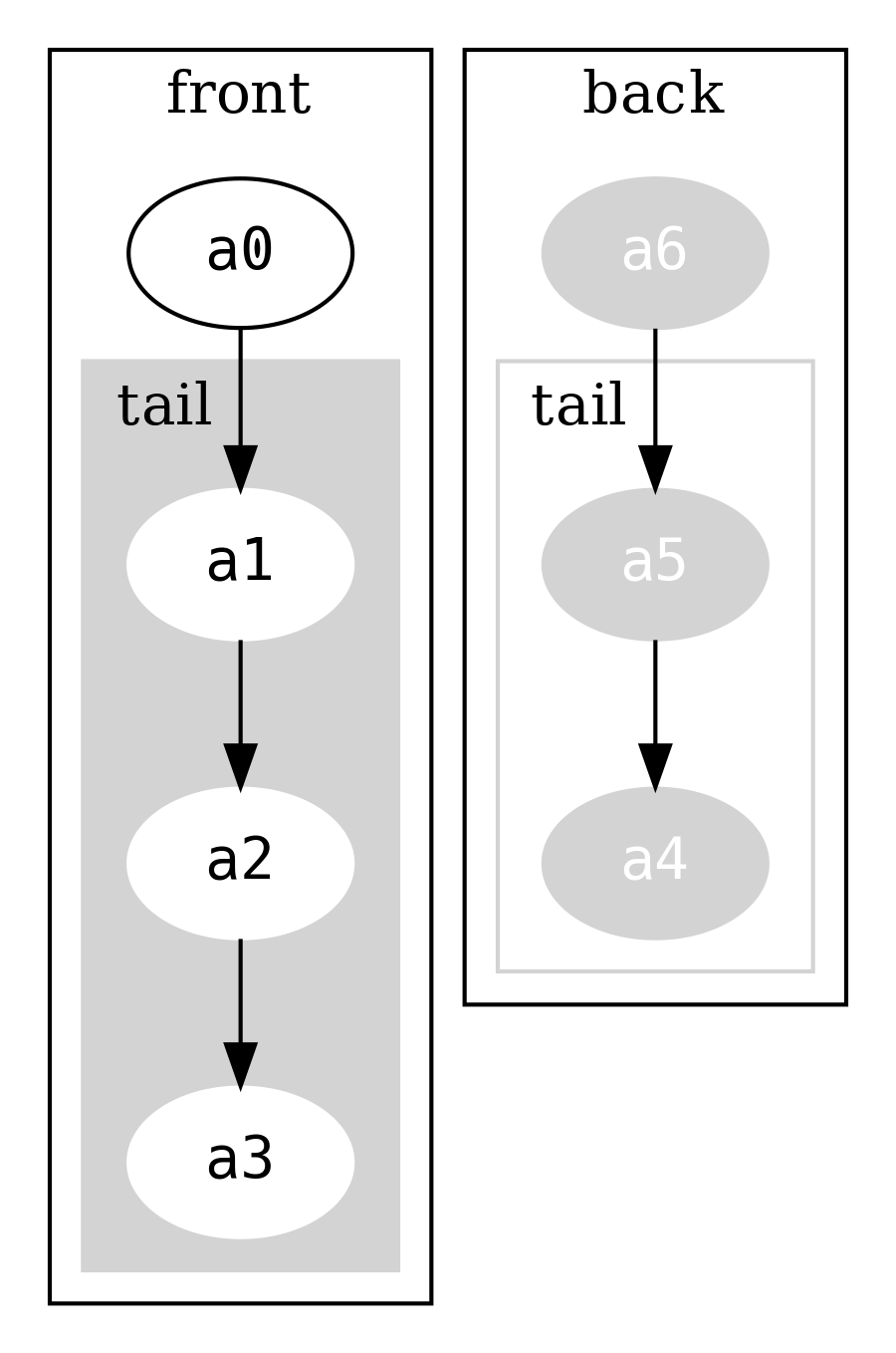
Note that the list holding the back is in reverse order.

Reading the snoc (final element) is a simple lookup into back.head. Adding an element to the end of the Dequeue means adding a new element to the head of the back, and recreating the FullDequeue wrapper (which will increase backSize by one). Almost all of the original structure is shared. Compare to adding a new element to the end of an IList, which would involve recreating the entire structure.

The frontSize and backSize are used to re-balance the front and back so that they are always approximately the same size. Re-balancing means that some operations can be slower than others (e.g. when the entire structure must be rebuilt) but because it happens only occasionally, we can take the average of the cost and say that it is constant.

6.8.6 DList

Linked lists have poor performance characteristics when large lists are appended together. Consider the work that goes into evaluating the following:

  ((as ::: bs) ::: (cs ::: ds)) ::: (es ::: (fs ::: gs))

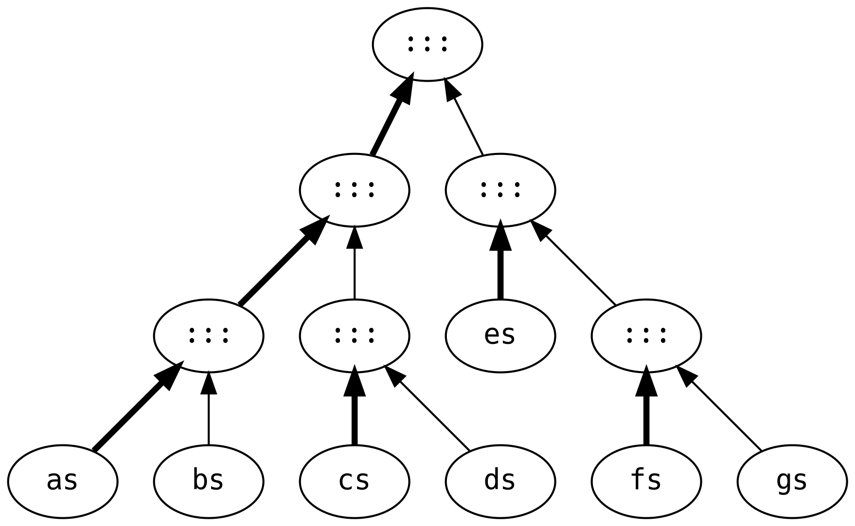
This creates six intermediate lists, traversing and rebuilding every list three times (except for gs which is shared between all stages).

The DList (for difference list) is a more efficient solution for this scenario. Instead of performing the calculations at each stage, it is represented as a function IList[A] => IList[A]

  final case class DList[A](f: IList[A] => IList[A]) {
    def toIList: IList[A] = f(IList.empty)
    def ++(as: DList[A]): DList[A] = DList(xs => f(as.f(xs)))
    ...
  }
  object DList {
    def fromIList[A](as: IList[A]): DList[A] = DList(xs => as ::: xs)
  }

The equivalent calculation is (the symbols created via DList.fromIList)

  (((a ++ b) ++ (c ++ d)) ++ (e ++ (f ++ g))).toIList

which breaks the work into right-associative (i.e. fast) appends

  (as ::: (bs ::: (cs ::: (ds ::: (es ::: (fs ::: gs))))))

utilising the fast constructor on IList.

As always, there is no free lunch. There is a memory allocation overhead that can slow down code that naturally results in right-associative appends. The largest speedup is when IList operations are left-associative, e.g.

  ((((((as ::: bs) ::: cs) ::: ds) ::: es) ::: fs) ::: gs)

Difference lists suffer from bad marketing. If they were called a ListBuilderFactory they’d probably be in the standard library.

6.8.7 ISet

Tree structures are excellent for storing ordered data, with every binary node holding elements that are less than in one branch, and greater than in the other. However, naive implementations of a tree structure can become unbalanced depending on the insertion order. It is possible to maintain a perfectly balanced tree, but it is incredibly inefficient as every insertion effectively rebuilds the entire tree.

ISet is an implementation of a tree of bounded balance, meaning that it is approximately balanced, using the size of each branch to balance a node.

  sealed abstract class ISet[A] {
    val size: Int = this match {
      case Tip()        => 0
      case Bin(_, l, r) => 1 + l.size + r.size
    }
    ...
  }
  object ISet {
    private final case class Tip[A]() extends ISet[A]
    private final case class Bin[A](a: A, l: ISet[A], r: ISet[A]) extends ISet[A]
  
    def empty[A]: ISet[A] = Tip()
    def singleton[A](x: A): ISet[A] = Bin(x, Tip(), Tip())
    def fromFoldable[F[_]: Foldable, A: Order](xs: F[A]): ISet[A] =
      xs.foldLeft(empty[A])((a, b) => a insert b)
    ...
  }

ISet requires A to have an Order. The Order[A] instance must remain the same between calls or internal assumptions will be invalid, leading to data corruption: i.e. we are assuming typeclass coherence such that Order[A] is unique for any A.

The ISet ADT unfortunately permits invalid trees. We strive to write ADTs that fully describe what is and isn’t valid through type restrictions, but sometimes there are situations where it can only be achieved by the inspired touch of an immortal. Instead, Tip / Bin are private, to stop users from accidentally constructing invalid trees. .insert is the only way to build an ISet, therefore defining what constitutes a valid tree.

  sealed abstract class ISet[A] {
    ...
    def contains(x: A)(implicit o: Order[A]): Boolean = ...
    def union(other: ISet[A])(implicit o: Order[A]): ISet[A] = ...
    def delete(x: A)(implicit o: Order[A]): ISet[A] = ...
  
    def insert(x: A)(implicit o: Order[A]): ISet[A] = this match {
      case Tip() => ISet.singleton(x)
      case self @ Bin(y, l, r) => o.order(x, y) match {
        case LT => balanceL(y, l.insert(x), r)
        case GT => balanceR(y, l, r.insert(x))
        case EQ => self
      }
    }
    ...
  }

The internal methods .balanceL and .balanceR are mirrors of each other, so we only study .balanceL, which is called when the value we are inserting is less than the current node. It is also called by the .delete method.

  def balanceL[A](y: A, left: ISet[A], right: ISet[A]): ISet[A] = (left, right) match {
  ...

Balancing requires us to classify the scenarios that can occur. We will go through each possible scenario, visualising the (y, left, right) on the left side of the page, with the balanced structure on the right, also known as the rotated tree.

• filled circles visualise a Tip
• three columns visualise the left | value | right fields of Bin
• diamonds visualise any ISet

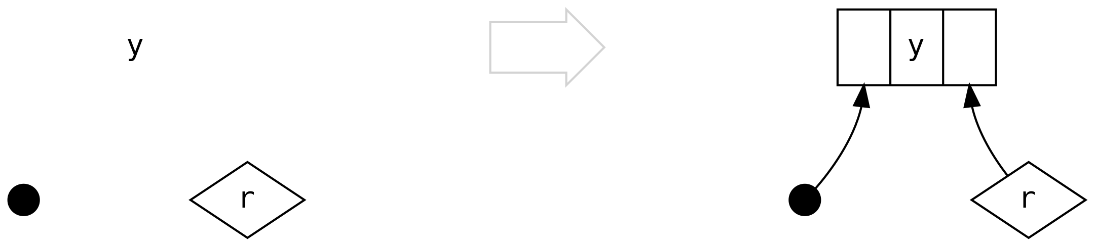
The first scenario is the trivial case, which is when both the left and right are Tip. In fact we will never encounter this scenario from .insert, but we hit it in .delete

  case (Tip(), Tip()) => singleton(y)

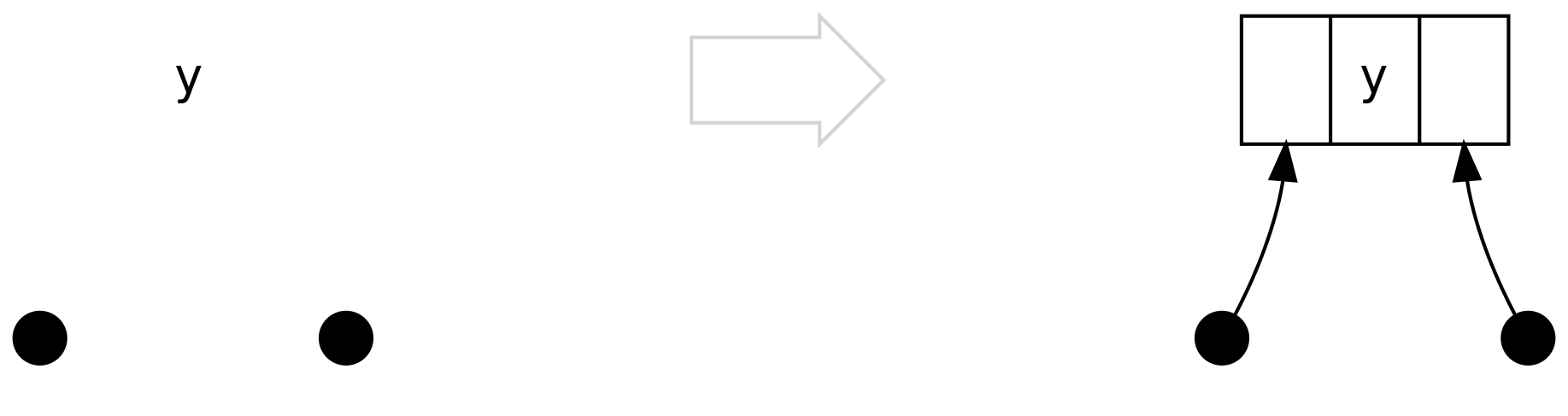
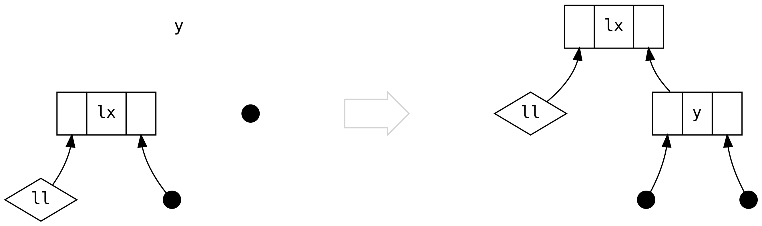
The second case is when left is a Bin containing only Tip, we don’t need to balance anything, we just create the obvious connection:

  case (Bin(lx, Tip(), Tip()), Tip()) => Bin(y, left, Tip())

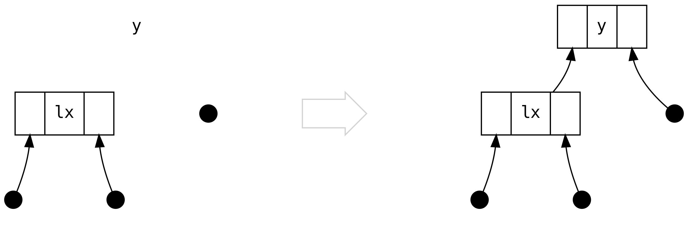
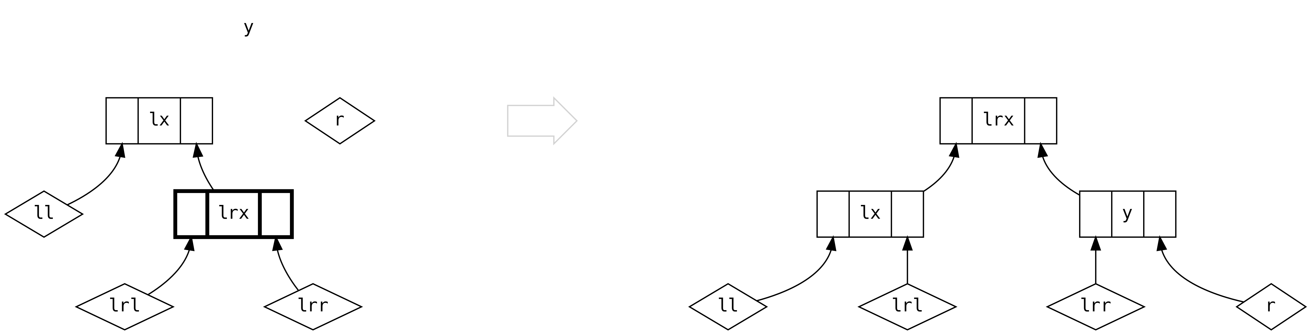
The third case is when it starts to get interesting: left is a Bin containing a Bin in its right

  case (Bin(lx, Tip(), Bin(lrx, _, _)), Tip()) =>
    Bin(lrx, singleton(lx), singleton(y))

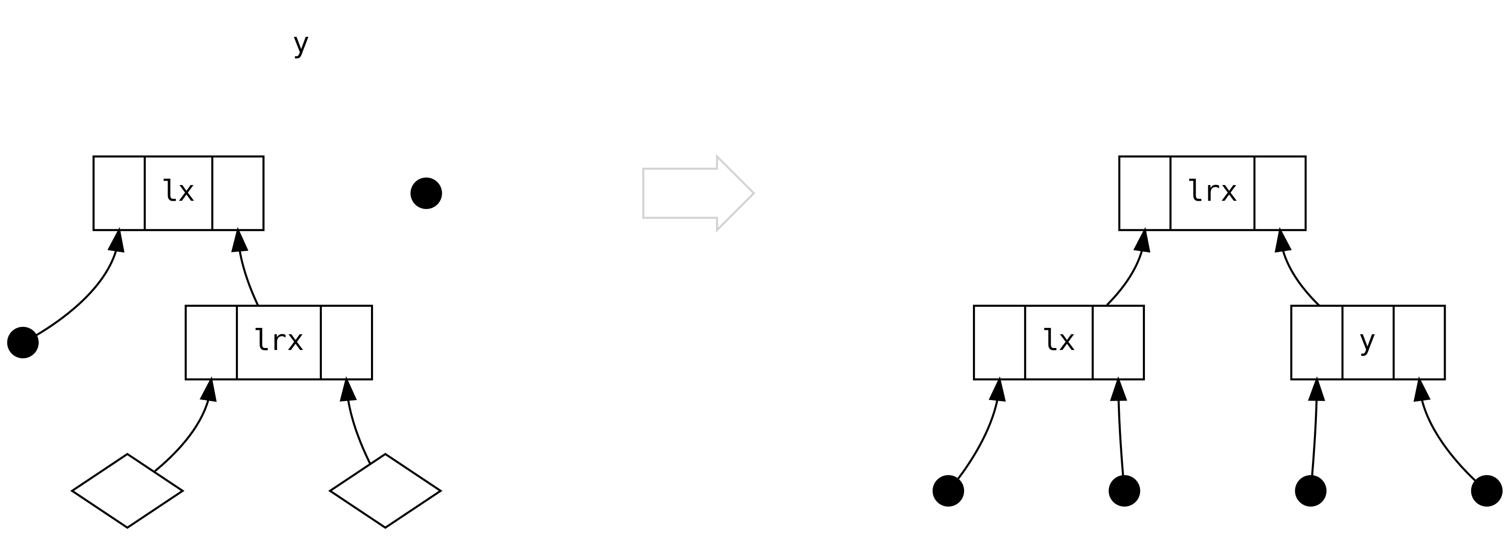
But what happened to the two diamonds sitting below lrx? Didn’t we just lose information? No, we didn’t lose information, because we can reason (based on size balancing) that they are always Tip! There is no rule in any of the following scenarios (or in .balanceR) that can produce a tree of the shape where the diamonds are Bin.

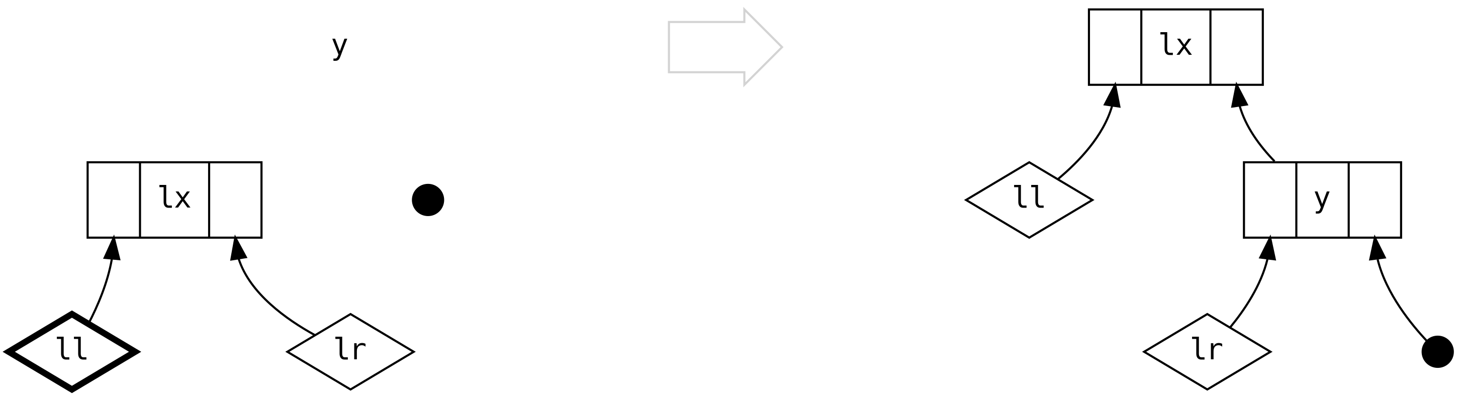
The fourth case is the opposite of the third case.

  case (Bin(lx, ll, Tip()), Tip()) => Bin(lx, ll, singleton(y))

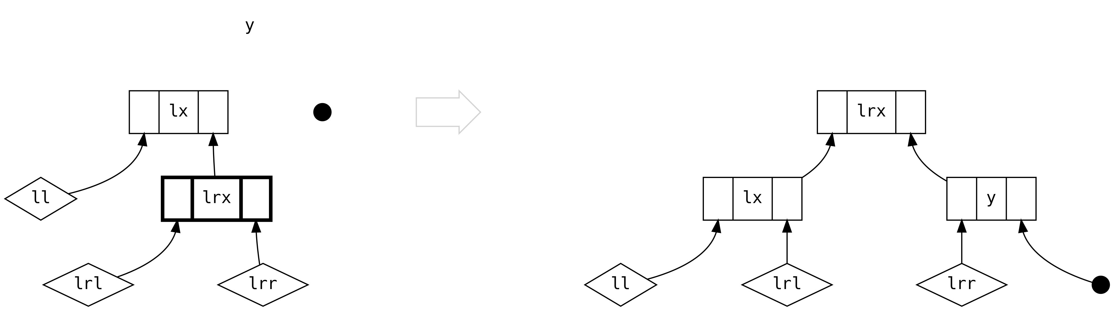
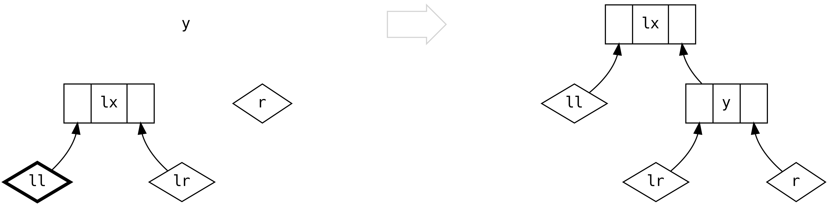
The fifth case is when we have full trees on both sides of the left and we must use their relative sizes to decide on how to re-balance.

  case (Bin(lx, ll, lr), Tip()) if (2*ll.size > lr.size) =>
    Bin(lx, ll, Bin(y, lr, Tip()))
  case (Bin(lx, ll, Bin(lrx, lrl, lrr)), Tip()) =>
    Bin(lrx, Bin(lx, ll, lrl), Bin(y, lrr, Tip()))

For the first branch, 2*ll.size > lr.size

and for the second branch 2*ll.size <= lr.size

The sixth scenario introduces a tree on the right. When the left is empty we create the obvious connection. This scenario never arises from .insert because the left is always non-empty:

  case (Tip(), r) => Bin(y, Tip(), r)

The final scenario is when we have non-empty trees on both sides. Unless the left is three times or more the size of the right, we can do the simple thing and create a new Bin

  case _ if l.size <= 3 * r.size => Bin(y, l, r)

However, should the left be more than three times the size of the right, we must balance based on the relative sizes of ll and lr, like in scenario five.

  case (Bin(lx, ll, lr), r) if (2*ll.size > lr.size) =>
    Bin(lx, ll, Bin(y, lr, r))
  case (Bin(lx, ll, Bin(lrx, lrl, lrr)), r) =>
    Bin(lrx, Bin(lx, ll, lrl), Bin(y, lrr, r))

This concludes our study of the .insert method and how the ISet is constructed. It should be of no surprise that Foldable is implemented in terms of depth-first search along the left or right, as appropriate. Methods such as .minimum and .maximum are optimal because the data structure already encodes the ordering.

It is worth noting that some typeclass methods cannot be implemented as efficiently as we would like. Consider the signature of Foldable.element

  @typeclass trait Foldable[F[_]] {
    ...
    def element[A: Equal](fa: F[A], a: A): Boolean
    ...
  }

The obvious implementation for .element is to defer to (almost) binary-search ISet.contains. However, it is not possible because .element provides Equal whereas .contains requires Order.

ISet is unable to provide a Functor for the same reason. In practice this turns out to be a sensible constraint: performing a .map would involve rebuilding the entire structure. It is sensible to convert to some other datatype, such as IList, perform the .map, and convert back. A consequence is that it is not possible to have Traverse[ISet] or Applicative[ISet].

6.8.8 IMap

  sealed abstract class ==>>[A, B] {
    val size: Int = this match {
      case Tip()           => 0
      case Bin(_, _, l, r) => 1 + l.size + r.size
    }
  }
  object ==>> {
    type IMap[A, B] = A ==>> B
  
    private final case class Tip[A, B]() extends (A ==>> B)
    private final case class Bin[A, B](
      key: A,
      value: B,
      left: A ==>> B,
      right: A ==>> B
    ) extends ==>>[A, B]
  
    def apply[A: Order, B](x: (A, B)*): A ==>> B = ...
  
    def empty[A, B]: A ==>> B = Tip[A, B]()
    def singleton[A, B](k: A, x: B): A ==>> B = Bin(k, x, Tip(), Tip())
    def fromFoldable[F[_]: Foldable, A: Order, B](fa: F[(A, B)]): A ==>> B = ...
    ...
  }

This is very familiar! Indeed, IMap (an alias to the lightspeed operator ==>>) is another size-balanced tree, but with an extra value: B field in each binary branch, allowing it to store key/value pairs. Only the key type A needs an Order and a suite of convenient methods are provided to allow easy entry updating

  sealed abstract class ==>>[A, B] {
    ...
    def adjust(k: A, f: B => B)(implicit o: Order[A]): A ==>> B = ...
    def adjustWithKey(k: A, f: (A, B) => B)(implicit o: Order[A]): A ==>> B = ...
    ...
  }

6.8.9 StrictTree and Tree

Both StrictTree and Tree are implementations of a Rose Tree, a tree structure with an unbounded number of branches in every node (unfortunately built from standard library collections for legacy reasons):

  case class StrictTree[A](
    rootLabel: A,
    subForest: Vector[StrictTree[A]]
  )

Tree is a by-need version of StrictTree with convenient constructors

  class Tree[A](
    rootc: Need[A],
    forestc: Need[Stream[Tree[A]]]
  ) {
    def rootLabel = rootc.value
    def subForest = forestc.value
  }
  object Tree {
    object Node {
      def apply[A](root: =>A, forest: =>Stream[Tree[A]]): Tree[A] = ...
    }
    object Leaf {
      def apply[A](root: =>A): Tree[A] = ...
    }
  }

The user of a Rose Tree is expected to manually balance it, which makes it suitable for cases where it is useful to encode domain knowledge of a hierarchy into the data structure. For example, in artificial intelligence, a Rose Tree can be used in clustering algorithms to organise data into a hierarchy of increasingly similar things. It is possible to represent XML documents with a Rose Tree.

If you find yourself working with hierarchical data, consider using a Rose Tree instead of rolling a custom data structure.

6.8.10 FingerTree

Finger trees are generalised sequences with amortised constant cost lookup and logarithmic concatenation. A is the type of data and it may help to ignore V:

  sealed abstract class FingerTree[V, A] {
    def +:(a: A): FingerTree[V, A] = ...
    def :+(a: =>A): FingerTree[V, A] = ...
    def <++>(right: =>FingerTree[V, A]): FingerTree[V, A] = ...
    ...
  }
  object FingerTree {
    private class Empty[V, A]() extends FingerTree[V, A]
    private class Single[V, A](v: V, a: =>A) extends FingerTree[V, A]
    private class Deep[V, A](
      v: V,
      left: Finger[V, A],
      spine: =>FingerTree[V, Node[V, A]],
      right: Finger[V, A]
    ) extends FingerTree[V, A]
  
    sealed abstract class Finger[V, A]
    final case class One[V, A](v: V, a1: A) extends Finger[V, A]
    final case class Two[V, A](v: V, a1: A, a2: A) extends Finger[V, A]
    final case class Three[V, A](v: V, a1: A, a2: A, a3: A) extends Finger[V, A]
    final case class Four[V, A](v: V, a1: A, a2: A, a3: A, a4: A) extends Finger[V, A]
  
    sealed abstract class Node[V, A]
    private class Node2[V, A](v: V, a1: =>A, a2: =>A) extends Node[V, A]
    private class Node3[V, A](v: V, a1: =>A, a2: =>A, a3: =>A) extends Node[V, A]
    ...
  }

Visualising FingerTree as dots, Finger as boxes and Node as boxes within boxes:

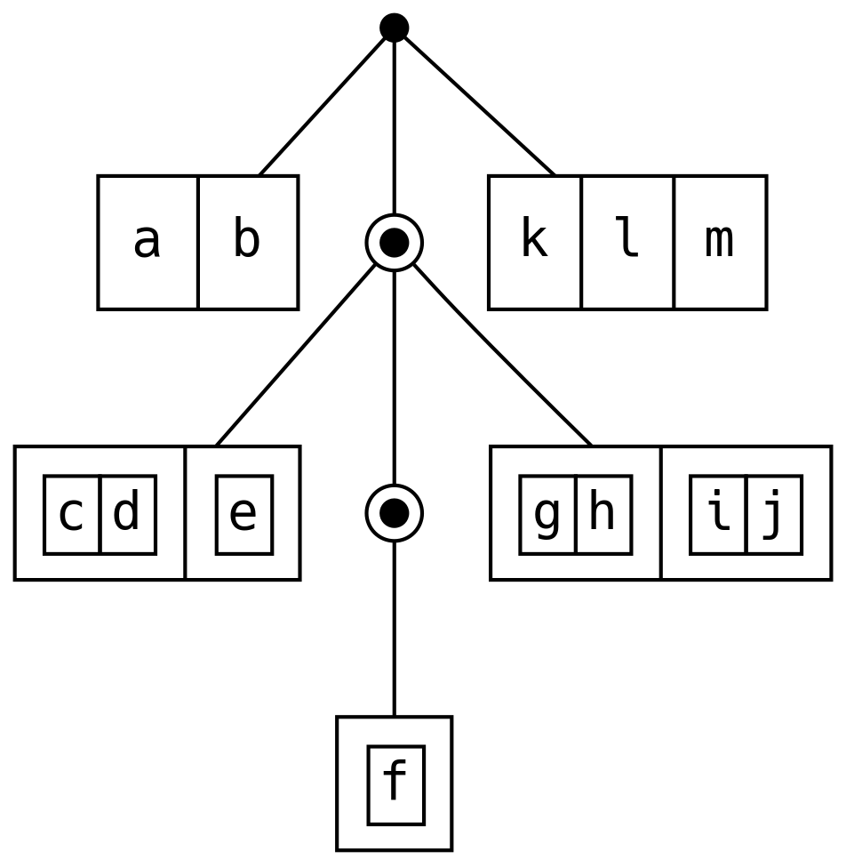
Adding elements to the front of a FingerTree with +: is efficient because Deep simply adds the new element to its left finger. If the finger is a Four, we rebuild the spine to take 3 of the elements as a Node3. Adding to the end, :+, is the same but in reverse.

Appending |+| (also <++>) is more efficient than adding one element at a time because the case of two Deep trees can retain the outer branches, rebuilding the spine based on the 16 possible combinations of the two Finger values in the middle.

In the above we skipped over V. Not shown in the ADT description is an implicit measurer: Reducer[A, V] on every element of the ADT.

Reducer is an extension of Monoid that allows for single elements to be added to an M

  class Reducer[C, M: Monoid] {
    def unit(c: C): M
  
    def snoc(m: M, c: C): M = append(m, unit(c))
    def cons(c: C, m: M): M = append(unit(c), m)
  }

For example, Reducer[A, IList[A]] can provide an efficient .cons

  implicit def reducer[A]: Reducer[A, IList[A]] = new Reducer[A, IList[A]] {
    override def unit(a: A): IList[A] = IList.single(a)
    override def cons(a: A, as: IList[A]): IList[A] = a :: as
  }

6.8.10.1 IndSeq

If we use Int as V, we can get an indexed sequence, where the measure is size, allowing us to perform index-based lookup by comparing the desired index with the size at each branch in the structure:

  final class IndSeq[A](val self: FingerTree[Int, A])
  object IndSeq {
    private implicit def sizer[A]: Reducer[A, Int] = _ => 1
    def apply[A](as: A*): IndSeq[A] = ...
  }

Another use of FingerTree is as an ordered sequence, where the measure stores the largest value contained by each branch:

6.8.10.2 OrdSeq

  final class OrdSeq[A: Order](val self: FingerTree[LastOption[A], A]) {
    def partition(a: A): (OrdSeq[A], OrdSeq[A]) = ...
    def insert(a: A): OrdSeq[A] = ...
    def ++(xs: OrdSeq[A]): OrdSeq[A] = ...
  }
  object OrdSeq {
    private implicit def keyer[A]: Reducer[A, LastOption[A]] = a => Tag(Some(a))
    def apply[A: Order](as: A*): OrdSeq[A] = ...
  }

OrdSeq has no typeclass instances so it is only useful for incrementally building up an ordered sequence, with duplicates. We can access the underlying FingerTree when needed.

6.8.10.3 Cord

The most common use of FingerTree is as an efficient intermediate holder for String representations in Show. Building a single String can be thousands of times faster than the default case class implementation of nested .toString, which builds a String for every layer in the ADT.

  final case class Cord(self: FingerTree[Int, String]) {
    override def toString: String = {
      val sb = new java.lang.StringBuilder(self.measure)
      self.foreach(sb.append) // locally scoped side effect
      sb.toString
    }
    ...
  }

For example, the Cord[String] instance returns a Three with the string in the middle and quotes on either side

  implicit val show: Show[String] = s => Cord(FingerTree.Three("\"", s, "\""))

Therefore a String renders as it is written in source code

  scala> val s = "foo"
         s.toString
  res: String = foo
  
  scala> s.show
  res: Cord = "foo"

6.8.11 Heap Priority Queue

A priority queue is a data structure that allows fast insertion of ordered elements, allowing duplicates, with fast access to the minimum value (highest priority). The structure is not required to store the non-minimal elements in order. A naive implementation of a priority queue could be

  final case class Vip[A] private (val peek: Maybe[A], xs: IList[A]) {
    def push(a: A)(implicit O: Order[A]): Vip[A] = peek match {
      case Maybe.Just(min) if a < min => Vip(a.just, min :: xs)
      case _                          => Vip(peek, a :: xs)
    }
  
    def pop(implicit O: Order[A]): Maybe[(A, Vip[A])] = peek strengthR reorder
    private def reorder(implicit O: Order[A]): Vip[A] = xs.sorted match {
      case INil()           => Vip(Maybe.empty, IList.empty)
      case ICons(min, rest) => Vip(min.just, rest)
    }
  }
  object Vip {
    def fromList[A: Order](xs: IList[A]): Vip[A] = Vip(Maybe.empty, xs).reorder
  }

This push is a very fast O(1), but reorder (and therefore pop) relies on IList.sorted costing O(n log n).

Scalaz encodes a priority queue, with a tree structure where every node has a value less than its children, called a Heap Priority Queue. Heap has fast push (insert), union, size, pop (uncons) and peek (minimumO) operations:

  sealed abstract class Heap[A] {
    def insert(a: A)(implicit O: Order[A]): Heap[A] = ...
    def +(a: A)(implicit O: Order[A]): Heap[A] = insert(a)
  
    def union(as: Heap[A])(implicit O: Order[A]): Heap[A] = ...
  
    def uncons(implicit O: Order[A]): Option[(A, Heap[A])] = minimumO strengthR deleteMin
    def minimumO: Option[A] = ...
    def deleteMin(implicit O: Order[A]): Heap[A] = ...
  
    ...
  }
  object Heap {
    def fromData[F[_]: Foldable, A: Order](as: F[A]): Heap[A] = ...
  
    private final case class Ranked[A](rank: Int, value: A)
  
    private final case class Empty[A]() extends Heap[A]
    private final case class NonEmpty[A](
      size: Int,
      tree: Tree[Ranked[A]]
    ) extends Heap[A]
  
    ...
  }

Heap is implemented with a Rose Tree of Ranked values, where the rank is the depth of a subtree, allowing us to depth-balance the tree. We manually maintain the tree so the minimum value is at the top. An advantage of encoding the minimum value in the data structure is that minimumO (also known as peek) is a free lookup:

  def minimumO: Option[A] = this match {
    case Empty()                        => None
    case NonEmpty(_, Tree.Node(min, _)) => Some(min.value)
  }

When inserting a new entry, we compare to the current minimum and replace if the new entry is lower:

  def insert(a: A)(implicit O: Order[A]): Heap[A] = this match {
    case Empty() =>
      NonEmpty(1, Tree.Leaf(Ranked(0, a)))
    case NonEmpty(size, tree @ Tree.Node(min, _)) if a <= min.value =>
      NonEmpty(size + 1, Tree.Node(Ranked(0, a), Stream(tree)))
  ...

Insertions of non-minimal values result in an unordered structure in the branches of the minimum. When we encounter two or more subtrees of equal rank, we optimistically put the minimum to the front:

  ...
    case NonEmpty(size, Tree.Node(min,
           (t1 @ Tree.Node(Ranked(r1, x1), xs1)) #::
           (t2 @ Tree.Node(Ranked(r2, x2), xs2)) #:: ts)) if r1 == r2 =>
      lazy val t0 = Tree.Leaf(Ranked(0, a))
      val sub =
        if (x1 <= a && x1 <= x2)
          Tree.Node(Ranked(r1 + 1, x1), t0 #:: t2 #:: xs1)
        else if (x2 <= a && x2 <= x1)
          Tree.Node(Ranked(r2 + 1, x2), t0 #:: t1 #:: xs2)
        else
          Tree.Node(Ranked(r1 + 1, a), t1 #:: t2 #:: Stream())
  
      NonEmpty(size + 1, Tree.Node(Ranked(0, min.value), sub #:: ts))
  
    case NonEmpty(size,  Tree.Node(min, rest)) =>
      val t0 = Tree.Leaf(Ranked(0, a))
      NonEmpty(size + 1, Tree.Node(Ranked(0, min.value), t0 #:: rest))
  }

Avoiding a full ordering of the tree makes insert very fast, O(1), such that producers adding to the queue are not penalised. However, the consumer pays the cost when calling uncons, with deleteMin costing O(log n) because it must search for the minimum value, and remove it from the tree by rebuilding. That’s fast when compared to the naive implementation.

The union operation also delays ordering allowing it to be O(1).

If the Order[Foo] does not correctly capture the priority we want for the Heap[Foo], we can use Tag and provide a custom Order[Foo @@ Custom] for a Heap[Foo @@ Custom].

6.8.12 Diev (Discrete Intervals)

We can efficiently encode the (unordered) integer values 6, 9, 2, 13, 8, 14, 10, 7, 5 as inclusive intervals [2, 2], [5, 10], [13, 14]. Diev is an efficient encoding of intervals for elements A that have an Enum[A], getting more efficient as the contents become denser.

  sealed abstract class Diev[A] {
    def +(interval: (A, A)): Diev[A]
    def +(value: A): Diev[A]
    def ++(other: Diev[A]): Diev[A]
  
    def -(interval: (A, A)): Diev[A]
    def -(value: A): Diev[A]
    def --(other: Diev[A]): Diev[A]
  
    def intervals: Vector[(A, A)]
    def contains(value: A): Boolean
    def contains(interval: (A, A)): Boolean
    ...
  }
  object Diev {
    private final case class DieVector[A: Enum](
      intervals: Vector[(A, A)]
    ) extends Diev[A]
  
    def empty[A: Enum]: Diev[A] = ...
    def fromValuesSeq[A: Enum](values: Seq[A]): Diev[A] = ...
    def fromIntervalsSeq[A: Enum](intervals: Seq[(A, A)]): Diev[A] = ...
  }

When updating the Diev, adjacent intervals are merged (and then ordered) such that there is a unique representation for a given set of values.

  scala> Diev.fromValuesSeq(List(6, 9, 2, 13, 8, 14, 10, 7, 5))
  res: Diev[Int] = ((2,2)(5,10)(13,14))
  
  scala> Diev.fromValuesSeq(List(6, 9, 2, 13, 8, 14, 10, 7, 5).reverse)
  res: Diev[Int] = ((2,2)(5,10)(13,14))

A great usecase for Diev is for storing time periods. For example, in our TradeTemplate from the previous chapter

  final case class TradeTemplate(
    payments: List[java.time.LocalDate],
    ccy: Option[Currency],
    otc: Option[Boolean]
  )

if we find that the payments are very dense, we may wish to swap to a Diev representation for performance reasons, without any change in our business logic because we used Monoid, not any List specific methods. We would, however, have to provide an Enum[LocalDate], which is an otherwise useful thing to have.

6.8.13 OneAnd

Recall that Foldable is the scalaz equivalent of a collections API and Foldable1 is for non-empty collections. So far we have only seen NonEmptyList to provide a Foldable1. The simple data structure OneAnd wraps any other collection to turn it into a Foldable1:

  final case class OneAnd[F[_], A](head: A, tail: F[A])

NonEmptyList[A] could be an alias to OneAnd[IList, A]. Similarly, we can create non-empty Stream, DList and Tree structures. However it may break ordering and uniqueness characteristics of the underlying structure: a OneAnd[ISet, A] is not a non-empty ISet, it is an ISet with a guaranteed first element that may also be in the ISet.

6.9 Summary

In this chapter we have skimmed over the data types that scalaz has to offer.

It is not necessary to remember everything in this chapter: think of each section as having planted the kernel of an idea in your mind. If, in a few months, you find yourself thinking “I remember reading about a data structure that might be useful here” and you return to these pages, we have succeeded.

The world of functional data structures is an active area of research. Academic publications appear regularly with new approaches to old problems. If you are the kind of person who would like to contribute back to scalaz, finding a functional data structure to implement would be greatly appreciated.