Leanpub: Publish Early, Publish Often

Use Case: MNIST Digit Classification

MNIST Overview

The MNIST database is a famous academic dataset used to benchmark classification performance. The data consists of 60,000 training images and 10,000 test images, each a standardized 28^2 pixel greyscale image of a single handwritten digit. You can download the datasets from the H2O GitHub repository for the H2O Deep Learning documentation. Remember to save these .csv files to your working directory. Following the weather data example, we begin by loading these datasets into R as H2OParsedData objects.

1 train_images.hex = h2o.uploadFile(h2o_server, path = "mnist_train.csv", header =\
2  FALSE, sep = ",", key = "train_images.hex")
3 test_images.hex = h2o.uploadFile(h2o_server, path = "mnist_test.csv", header = F\
4 ALSE, sep = ",", key = "test_images.hex")

Performing a Trial Run

The trial run below is illustrative of the relative simplicity that underlies most H2O Deep Learning model parameter configurations, thanks to the defaults. We use the first 28^2 = 784 values of each row to represent the full image, and the final value to denote the digit class. As mentioned before, Rectified linear activation is popular with image processing and has performed well on the MNIST database previously; and dropout has been known to enhance performance on this dataset as well – so we train our model accordingly.

1 #Train the model for digit classification
2 mnist_model = h2o.deeplearning(x = 1:784, y = 785, data = train_images.hex, acti\
3 vation = "RectifierWithDropout", hidden = c(200,200,200), input_dropout_ratio = \
4 0.2, l1 = 1e-5, validation = test_images.hex, epochs = 10)

The model is run for only 10 epochs since it is meant just as a trial run. In this trial run we also specified the validation set to be the test set, but another option is to use n-fold validation by specifying, for example, nfolds=5 instead of validation=test_images.

Extracting and Handling the Results

We can extract the parameters of our model, examine the scoring process, and make predictions on new data.

1 #View the specified parameters of your deep learning model
2 mnist_model@model$params
3 
4 #Examine the performance of the trained model
5 mnist_model

The latter command returns the trained model’s training and validation error. The training error value is based on the parameter score_training_samples, which specifies the number of randomly sampled training points to be used for scoring; the default uses 10,000 points. The validation error is based on the parameter score_validation_samples, which controls the same value on the validation set and is set by default to be the entire validation set. In general choosing more sampled points leads to a better idea of the model’s performance on your dataset; setting either of these parameters to 0 automatically uses the entire corresponding dataset for scoring. Either way, however, you can control the minimum and maximum time spent on scoring with the score_interval and score_duty_cycle parameters.

These scoring parameters also affect the final model when the parameter override_with_best_model is turned on. This override sets the final model after training to be the model which achieved the lowest validation error during training, based on the sampled points used for scoring. Since the validation set is automatically set to be the training data if no other dataset is specified, either the score_training_samples or score_validation_samples parameter will control the error computation during training and, in turn, the chosen best model.

Once we have a satisfactory model, the h2o.predict() command can be used to compute and store predictions on new data, which can then be used for further tasks in the interactive data science process.

1 #Perform classification on the test set
2 prediction = h2o.predict(mnist_model, newdata=test_images.hex)
3 
4 #Copy predictions from H2O to R
5 pred = as.data.frame(prediction)

Web Interface

H2O R users have access to a slick web interface to mirror the model building process in R. After loading data or training a model in R, point your browser to your IP address and port number (e.g., localhost:12345) to launch the web interface. From here you can click on $\textsc{Admin}$ > $\textsc{Jobs}$ to view your specific model details. You can also click on $\textsc{Data}$ > $\textsc{View All}$ to view and keep track of your datasets in current use.

Variable Importances

One useful feature is the variable importances option, which can be enabled with the additional argument variable_importances=TRUE. This features allows us to view the absolute and relative predictive strength of each feature in the prediction task. From R, you can access these strengths with the command mnist_model@model$varimp. You can also view a visualization of the variable importances on the web interface.

Java Models

Another important feature of the web interface is the Java (POJO) model, accessible from the $\textsc{Java model}$ button in the top right of a model summary page. This button allows access to Java code which, when called from a main method in a Java program, builds the model. Instructions for downloading and running this Java code are available from the web interface, and example production scoring code is available as well.

Grid Search for Model Comparison

H2O supports grid search capabilities for model tuning by allowing users to tweak certain parameters and observe changes in model behavior. This is done by specifying sets of values for parameter arguments. For example, below is an example of a grid search:

1 #Create a set of network topologies
2 hidden_layers = list(c(200,200), c(100,300,100),c(500,500,500))
3 
4 mnist_model_grid = h2o.deeplearning(x = 1:784, y = 785, data = train_images.hex,\
5  activation = "RectifierWithDropout", hidden = hidden_layers, validation = test_\
6 images.hex, epochs = 1, l1 = c(1e-5,1e-7), input_dropout_ratio = 0.2)

Here we specified three different network topologies and two different $\ell_1$ norm weights. This grid search model effectively trains six different models, over the possible combinations of these parameters. Of course, sets of other parameters can be specified for a larger space of models. This allows for more subtle insights in the model tuning and selection process, as we inspect and compare our trained models after the grid search process is complete. To decide how and when to choose different parameter configurations in a grid search, see Appendix A for parameter descriptions and possible values.

 1 #print out all prediction errors and run times of the models
 2 mnist_model_grid
 3 mnist_model_grid@model
 4 
 5 #print out a *short* summary of each of the models (indexed by parameter)
 6 mnist_model_grid@sumtable
 7 
 8 #print out *full* summary of each of the models
 9 all_params = lapply(mnist_model_grid@model, function(x) { x@model$params })
10 all_params
11 
12 #access a particular parameter across all models
13 l1_params = lapply(mnist_model_grid@model, function(x) { x@model$params$l1 })
14 l1_params

Checkpoint Models

Checkpoint model keys can be used to start off where you left off, if you feel that you want to further train a particular model with more iterations, more data, different data, and so forth. If we felt that our initial model should be trained further, we can use it (or its key) as a checkpoint argument in a new model. In the command below, mnist_model_grid@model[[1]] indicates the highest performance model from the grid search that we wish to train further. Note that the training and validation datasets and the response column etc. have to match for checkpoint restarts.

1 mnist_checkpoint_model = h2o.deeplearning(x=1:784, y=785, data=train_images.hex,\
2  checkpoint=mnist_model_grid@model[[1]], validation = test_images.hex, epochs=9)

Checkpoint models are also applicable for the case when we wish to reload existing models that were saved to disk in a previous session. For example, we can save and later load the best model from the grid search by running the following commands.

1 #Specify a model and the file path where it is to be saved
2 h2o.saveModel(object = mnist_model_grid@model[[1]], name = "/tmp/mymodel", force\
3  = TRUE)
4 
5 #Alternatively, save the model key in some directory (here we use /tmp)
6 #h2o.saveModel(object = mnist_model_grid@model[[1]], dir = "/tmp", force = TRUE)

Later (e.g., after restarting H2O) we can load the saved model by indicating the host and saved model file path. This assumes the saved model was saved with a compatible H2O version (no changes to the H2O model implementation).

1 best_mnist_grid.load = h2o.loadModel(h2o_server, "/tmp/mymodel")
2 
3 #Continue training the loaded model
4 best_mnist_grid.continue = h2o.deeplearning(x=1:784, y=785, data=train_images.he\
5 x, checkpoint=best_mnist_grid.load, validation = test_images.hex, epochs=1)

Additionally, you can also use the command model = h2o.getModel(h2o_server, key) to retrieve a model from its H2O key. This command is useful, for example, if you have created an H2O model using the web interface and wish to proceed with the modeling process in R.

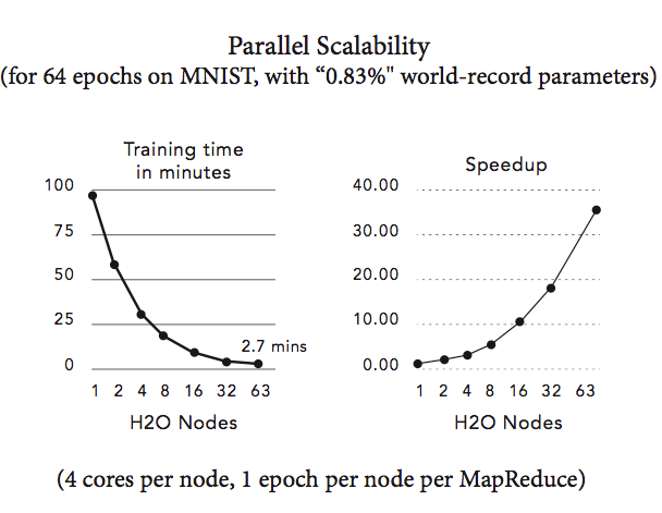
Achieving World Record Performance

Without distortions, convolutions, or other advanced image processing techniques, the best-ever published test set error for the MNIST dataset is 0.83% by Microsoft. After training for 2,000 epochs (took about 4 hours) on 4 compute nodes, we obtain 0.87% test set error and after training for 8,000 epochs (took about 10 hours) on 10 nodes, we obtain 0.83% test set error, which is the current world-record, notably achieved using a distributed configuration and with a simple 1-liner from R. Details can be found in our hands-on tutorial. Accuracies around 1% test set errors are typically achieved within 1 hour when running on 1 node. The parallel scalability of H2O for the MNIST dataset on 1 to 63 compute nodes is shown in the figure below.