H2O’s Deep Learning Architecture
As described above, H2O follows the model of multi-layer, feedforward neural networks for predictive modeling. This section provides a more detailed description of H2O’s Deep Learning features, parameter configurations, and computational implementation.
Summary of Features
H2O’s Deep Learning functionalities include:
- purely supervised training protocol for regression and classification tasks
- fast and memory-efficient Java implementations based on columnar compression and fine-grain Map/Reduce
- multi-threaded and distributed parallel computation to be run on either a single node or a multi-node cluster
- fully automatic per-neuron adaptive learning rate for fast convergence
- optional specification of learning rate, annealing and momentum options
- regularization options include L1, L2, dropout, Hogwild! and model averaging to prevent model overfitting
- elegant web interface or fully scriptable R API from H2O CRAN package
- grid search for hyperparameter optimization and model selection
- model checkpointing for reduced run times and model tuning
- automatic data pre and post-processing for categorical and numerical data
- automatic imputation of missing values
- automatic tuning of communication vs computation for best performance
- model export in plain java code for deployment in production environments
- additional expert parameters for model tuning
- deep autoencoders for unsupervised feature learning and anomaly detection capabilities
Training Protocol
The training protocol described below follows many of the ideas and advances in the recent deep learning literature.
Initialization
Various deep learning architectures employ a combination of unsupervised pretraining followed by supervised training, but H2O uses a purely supervised training protocol. The default initialization scheme is the uniform adaptive option, which is an optimized initialization based on the size of the network. Alternatively, you may select a random initialization to be drawn from either a uniform or normal distribution, for which a scaling parameter may be specified as well.
Activation and Loss Functions
In the introduction we introduced the nonlinear activation function  , for which the choices are summarized in Table 1. Note here that
  and
and  denote the firing neuron’s input values and their weights, respectively;
  denotes the weighted combination
 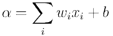 .
.
Table 1
| Function | Formula | Range |
| Tanh | 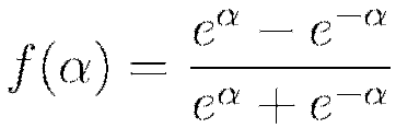 |
![f(\cdot) \in [-1,1]](/preview_site_images/deeplearning/leanpub_equation_22.png) |
| Rectified Linear | 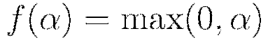 |
 |
| Maxout |  |
![f(\cdot) \in [-\infty,1]](/preview_site_images/deeplearning/leanpub_equation_26.png) |
The  function is a rescaled and shifted logistic function and its symmetry around 0 allows the training algorithm to converge faster. The rectified linear activation function has demonstrated high performance on image recognition tasks, and is a more biologically accurate model of neuron activations (LeCun et al, 1998). Maxout activation works particularly well with dropout, a regularization method discussed later in this vignette (Goodfellow et al, 2013). It is difficult to determine a “best” activation function to use; each may outperform the others in separate scenarios, but grid search models (also described later) can help to compare activation functions and other parameters. The default activation function is the Rectifier. Each of these activation functions can be operated with dropout regularization (see below).
The following choices for the loss function  are summarized in Table 2. The system default enforces the table’s typical use rule based on whether regression or classification is being performed. Note here that
  and
and  are the predicted (target) output and actual output, respectively, for training example
  ; further, let
  denote the output units and
  the output layer.
Table 2
| Function | Formula | Typical Use |
| Mean Squared Error | 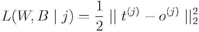 |
Regression |
| Cross Entropy | 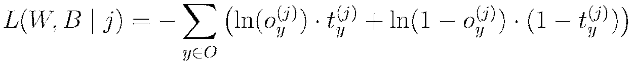 |
Classification |
Parallel Distributed Network Training
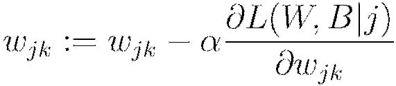
The procedure to minimize the loss function  is a parallelized version of stochastic gradient descent (SGD). Standard SGD can be summarized as follows, with the gradient
  computed via backpropagation (LeCun et al, 1998). The constant
  indicates the learning rate, which controls the step sizes during gradient descent.
Standard Stochastic Gradient Descent
Initialize 
Iterate until convergence criterion reached
Get training example 
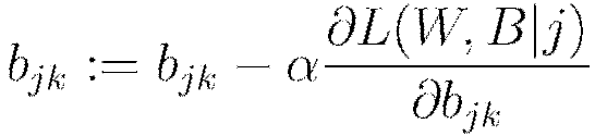
Update all weights  , biases

Stochastic gradient descent is known to be fast and memory-efficient, but not easily parallelizable without becoming slow. We utilize  , the recently developed lock-free parallelization scheme from (Niu et al, 2011).
  follows a shared memory model where multiple cores, each handling separate subsets (or all) of the training data, are able to make independent contributions to the gradient updates
  asynchronously. In a multi-node system this parallelization scheme works on top of H2O’s distributed setup, where the training data is distributed across the cluster. Each node operates in parallel on its local data until the final parameters
  are obtained by averaging. Below is a rough summary.
Parallel distributed and multi-threaded training with SGD in H2O Deep Learning
Initialize global model parameters 
Distribute training data  across nodes (can be disjoint or replicated)
Iterate until convergence criterion reached
For nodes  with training subset
  , do in parallel:
Obtain copy of the global model parameters 
Select active subset  (user-given number of samples per iteration)
Partition  into
into  by cores
For cores  on node
  , do in parallel:
Get training example 
Update all weights  , biases

Set 
Optionally score the model on (potentially sampled) train/validation scoring sets
Here, the weights and bias updates follow the asynchronous  procedure to incrementally adjust each node’s parameters
  after seeing example
  . The
. The  notation refers to the final averaging of these local parameters across all nodes to obtain the global model parameters and complete training.
Specifying the Number of Training Samples per Iteration
H2O Deep Learning is scalable and can take advantage of a large cluster of compute nodes. There are three modes in which to operate. The default behavior is to let every node train on the entire (replicated) dataset, but automatically locally shuffling (and/or using a subset of) the training examples for each iteration. For datasets that don’t fit into each node’s memory (also depending on the heap memory specified by the -Xmx option), it might not be possible to replicate the data, and each compute node can be instructed to train only with local data. An experimental single node mode is available for the case where slow final convergence is observed due to the presence of too many nodes, but we’ve never seen this become necessary.
The number of training examples (globally) presented to the distributed SGD worker nodes between model averaging is controlled by the important parameter train_samples_per_iteration. One special value is -1, which results in all nodes processing all their local training data per iteration. Note that if replicate_training_data is enabled (true by default), this will result in training N epochs (passes over the data) per iteration on N nodes, otherwise 1 epoch will be trained per iteration. Another special value is 0, which always results in 1 epoch per iteration, independent of the number of compute nodes. In general, any user-given positive number is permissible for this parameter. For large datasets, it might make sense to specify a fraction of the dataset.
For example, if the training data contains 10 million rows, and we specify the number of training samples per iteration as 100,000 when running on 4 nodes, then each node will process 25,000 examples per iteration, and it will take 40 such distributed iterations to process one epoch. If the value is set too high, it might take too long between synchronization and model convergence can be slow. If the value is set too low, network communication overhead will dominate the runtime, and computational performance will suffer. The special value of -2 (the default) enables auto-tuning of this parameter based on the computational performance of the processors and the network of the system and attempts to find a good balance between computation and communication. Note that this parameter can affect the convergence rate during training.
Regularization
H2O’s Deep Learning framework supports regularization techniques to prevent overfitting.
 and
and  regularization enforce the same penalties as they do with other models, that is, modifying the loss function so as to minimize some

For  regularization,
  represents of the sum of all
  norms of the weights and biases in the network;
  represents the sum of squares of all the weights and biases in the network. The constants
  and
and  are generally chosen to be very small, for example
  .
.
The second type of regularization available for deep learning is a recent innovation called dropout (Hinton et al., 2012).
Dropout constrains the online optimization such that during forward propagation for a given training example, each neuron in the network suppresses its activation with probability \textsc{P}, generally taken to be less than 0.2 for input neurons and up to 0.5 for hidden neurons. The effect is twofold: as with  regularization, the network weight values are scaled toward 0; furthermore, each training example trains a different model, albeit sharing the same global parameters. Thus dropout allows an exponentially large number of models to be averaged as an ensemble, which can prevent overfitting and improve generalization. Note that input dropout can be especially useful when the feature space is large and noisy.
Advanced Optimization
H2O features manual and automatic versions of advanced optimization. The manual mode features include momentum training and learning rate annealing, while automatic mode features adaptive learning rate.
Momentum Training
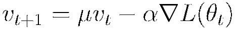
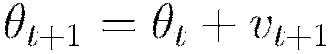
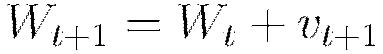
Momentum modifies back-propagation by allowing prior iterations to influence the current update. In particular, a velocity vector  is defined to modify the updates as follows, with
  representing the parameters
  ;
;  representing the momentum coefficient, and
  denoting the learning rate.
Using the momentum parameter can aid in avoiding local minima and the associated instability (Sutskever et al 2014). Too much momentum can lead to instabilities, which is why the momentum is best ramped up slowly.
A recommended improvement when using momentum updates is the Nesterov accelerated gradient method. Under this method the updates are further modified such that

Rate Annealing
Throughout training, as the model approaches a minimum the chance of oscillation or “optimum skipping” creates the need for a slower learning rate. Instead of specifying a constant learning rate  , learning rate annealing gradually reduces the learning rate
  to “freeze” into local minima in the optimization landscape (Zeiler, 2012).
For H2O, the annealing rate is the inverse of the number of training samples it takes to cut the learning rate in half (e.g.,  means that it takes
  training samples to halve the learning rate).
Adaptive Learning
The implemented adaptive learning rate algorithm ADADELTA (Zeiler, 2012) automatically combines the benefits of learning rate annealing and momentum training to avoid slow convergence. Specification of only two parameters  and
and  simplifies hyper parameter search. In some cases, manually controlled (non-adaptive) learning rate and momentum specifications can lead to better results, but require the hyper-parameter search of up to 7 parameters. If the model is built on a topology with many local minima or long plateaus, it is possible for a constant learning rate to produce sub-optimal results. In general, however, we find adaptive learning rate to produce the best results, and this option is kept as the default.
The first of two hyper parameters for adaptive learning is  . It is similar to momentum and relates to the memory to prior weight updates. Typical values are between 0.9 and 0.999. The second of two hyper parameters
  for adaptive learning is similar to learning rate annealing during initial training and momentum at later stages where it allows forward progress.
Typical values are between
for adaptive learning is similar to learning rate annealing during initial training and momentum at later stages where it allows forward progress.
Typical values are between  and
and  .
.
Loading Data
Loading a dataset in R for use with H2O is slightly different from the usual methodology, as we must convert our datasets into H2OParsedData objects. For an example, we use a toy weather dataset included in the H2O GitHub repository for the H2O Deep Learning documentation. First load the data to your current working directory in your R Console (do this henceforth for dataset downloads), and then run the following command.
weather.hex = h2o.uploadFile(h2o_server, path = "weather.csv", header = TRUE, sep = ",", key = "weather.hex"
To see a quick summary of the data, run the following command.
summary(weather.hex)
Input Standardization
Along with categorical encoding, H2O preprocesses data to be standardized for compatibility with the activation functions. Recall Table 1’s summary of each activation function’s target space. Since in general the activation function does not map into  , we first standardize our data to be drawn from
  . Standardizing again after network propagation allows us to compute more precise errors in this standardized space rather than in the raw feature space.
Additional Parameters
This section has reviewed some background on the various parameter configurations in H2O’s Deep Learning architecture. H2O Deep Learning models may seem daunting since there are dozens of possible parameter arguments when creating models. However, most parameters do not need to be tuned or experimented with; the default settings are safe and recommended. Those parameters for which experimentation is possible and perhaps necessary have mostly been discussed here but there a couple more which deserve mention.
There is no default for both hidden layer size/number as well as epochs. Practice building deep learning models with different network topologies and different datasets will lead to intuition for these parameters but two general rules of thumb should be applied. First, choose larger network sizes, as they can perform higher-level feature extraction, and techniques like dropout may train only subsets of the network at once. Second, use more epochs for greater predictive accuracy, but only when able to afford the computational cost. Many example tests can be found in the H2O GitHub repository for pointers on specific values and results for these (and other) parameters.
For a full list of H2O Deep Learning model parameters and default values, see Appendix A.