Chapter 4: Phylogenetic Community Ecology
4.1 Introduction
There is growing interest in using phylogenies to explore patterns of community composition – how species are distributed with respect to each other and with respect to environmental gradients in space. The distribution of species among communities depends in part on their traits. For example, in high-elevation habitats plant species that are tolerant of cold and snow are more likely to occur, and tolerance to cold winters depends on numerous adaptive traits. Similarly, fish species that are tolerant of low pH are more likely to occur in acidic lakes, and acid tolerance involves many fish traits. Since many traits are phylogenetically correlated among species, you would expect the distribution of species among communities to reflect, at least in part, phylogenies, with closely related species more likely to occur in similar communities. This is called phylogenetic attraction. Conversely, phylogenetically closely related species may be less likely to occur in the same communities. This might occur, for example, if closely related species with similar resource requirements are more likely to compete with each other, leaving only one present in a community. This pattern of phylogenetic repulsion could also arise through apparent competition with shared predators, with the more susceptible of a group of phylogenetically related prey species getting extirpated from communities by the predators. Thus, there are numerous ways in which phylogenies might be expected to be seen in patterns of community composition.
Phylogenetic community ecology uses the information available in phylogenetic relationships to understand community composition among spatially separated sites. Phylogenetic information is often used as a surrogate for missing information about variation in trait values among species, and missing information about how these traits affect the presence and abundance of species in communities. I am interested in the statistical problem of identifying these phylogenetic patterns. I think the problem of trying to infer the biological processes underlying these patterns is far more challenging. For example, if species show the pattern of phylogenetic repulsion, with closely related species less likely to occur in the same communities, I don’t think that this provides compelling evidence that competition is involved in structuring communities. However, it does give license for more detailed studies to see if competition is important. Phylogenies are also sometimes interpreted as surrogates for unmeasured traits: if there are phylogenetic patterns in community composition, then there must be traits underlying these patterns. I think this is likely to be correct, although it is necessary to be cautious, because the traits that you suspect are involved might in fact not be. My philosophy is to look for patterns and make sure they are statistically well-founded. If they are, then start the biological work to try to understand the processes driving the patterns.
Data on phylogenetic community composition are both hierarchical and phylogenetic. Therefore, the data are correlated. They combine characteristics of hierarchical data discussed in Chapters 1 and 2, and phylogenetic data discussed in Chapter 3. The approach I take (which should be no surprise) is to model the distribution of species among communities. There is also a rich history in community ecology of using metrics that measure a pattern of interest and then using permutation tests to determine if these patterns are statistically significant. This approach of using metrics and permutation tests can be very useful and powerful for simple problems. However, as problems become more complex, they become less useful and informative. Furthermore, because the metric approach does not produce fitted models that can simulate data, the results can be very difficult to assess: do the results really answer the questions you are asking? Building models for community composition is in some ways statistically more challenging, and requires greater computing power, but the payoff is greater flexibly in the questions that can be asked, and sometimes greater confidence in the answers.
This chapter presents models of phylogenetic community composition as a series of examples of increasing complexity. The models are mostly Phylogenetic Linear Mixed Models (PLMMs) that incorporate both hierarchical and phylogenetic covariance matrices into LMMs for continuous (abundance) data. At the end of the chapter I’ll also present Phylogenetic Generalized Linear Mixed Models (PGLMMs) for binary (presence/absence) data. The chapter explains how to construct and test models for a range of different types of problems. I’ll begin by asking whether there is phylogenetic signal in the composition of communities. Are phylogenetically related species more or less likely to occur in the same site? This question assumes you have no information about either traits shared by species or environmental differences among sites. The second question is related to the first. If you have information about environmental differences among sites, can you account for these differences to reveal phylogenetic patterns in the distribution of species that otherwise would be obscured. The third question is, if you have trait information about species but not about the environment, does this trait information explain the phylogenetic patterns in the distribution of species among sites. Answering this question requires a statistical test of whether the phylogenetic signal in the distribution of species is explained by a set of traits that you have measured. The fourth question assumes you have both trait and environmental information, and asks whether together these can explain the distribution of species among sites. Thus, the first four questions assume you do or don’t have trait and environmental information, in all 2-by-2 combinations.
The final question assumes that the sites themselves have a phylogeny. This is the case, for example, if the communities are pollinators and the sites are the plants they visit, with the plants having a phylogeny. Similar cases are diseases distributed among hosts, and predators attacking a smorgasbord of prey species. Questions that can be asked of such bipartite data (having two groups like pollinators and plants that interact with each other) include the presence of phylogenetic signal from one or both of the groups, and the role of traits in generating these phylogenetic signals.
I’ll address these five questions assuming that information is known about species abundances in each site. The questions could also be asked if only presence/absence of species in sites were known. Therefore, I’ll end the chapter with a re-examination of the first question using presence/absence (binary) data. Binary data for phylogenetic community composition involves the same issues that we have seen for binary data in hierarchical and phylogenetic data in Chapters 1-3: they contain less information than abundance data and introduce greater mathematical and computational challenges.
There are few statistical toolboxes for building models of phylogenetic community composition. This chapter relies heavily on the package phyr and its function communityPGLMM(). The math underlying this function was developed for fitting models of community composition (Ives and Helmus 2011) and then expanded to the case of bipartite phylogenies (Rafferty and Ives 2013). An older version of communityPGLMM() is in the package pez. Daijiang Li updated communityPGLMM() for phyr, and it has a nicer syntax and is much faster (running in C++). Also, Russell Dinnage has added Bayesian capabilities to communityPGLMM(), although I will use it only in frequentist mode. In some respects, this chapter serves as the manual for communityPGLMM().
4.2 Take-homes
- Phylogenetic models of community composition combine approaches for dealing with data having hierarchical structure and phylogenetic structure. Thus, PLMMs and PGLMMs incorporate two types of correlations in data.
- PGLMMs can explain the distribution of species among communities using only information about phylogenies. However, these models can also flexibly include information about traits shared by species and environmental factors shared by communities.
- Hierarchical and phylogenetic correlations present the same challenges as hierarchical data (Chapters 1 and 2) and phylogenetic data (Chapter 3). Failing to account for the correlated structure of the data can lead to inflated type I errors (false positives) or reduced power (false negatives).
- Phylogenetic community models can be used to test which traits and which environmental factors are responsible for phylogenetic patterns in the data. They can test hypotheses for why the phylogenetic patterns exist.
- Although PGLMMs provide flexible tools for testing a wide range of hypotheses in a diverse collection of community ecology data, there are limits to the size of datasets they can reasonably handle. For complex hypotheses involving many covariance patterns, fitting PGLMMs with more than 1000-2000 species-site data points will be computationally slow.
4.3 Phylogenetic patterns in community composition
The first question I’ll address is how to detect phylogenetic signal in the distribution of species among sites (communities) in the absence of information about trait characteristics of species and environmental characteristics of sites. To set up this problem, I’ll assume that species differ in mean abundance across all sites, that sites differ in the mean abundance of species they contain, and that there is phylogenetic attraction, with phylogenetically related species being more likely to occur in the same site. Below, I’ll first present the model and then investigate type I errors and statistical power.
4.3.1 A PLMM for phylogenetic attraction
The code for simulating and fitting a PLMM for phylogenetic attraction is similar to that for a LMM. Here, I’ll assume that abundances of species are known in every site, and Y gives these abundances, possibly transformed. I’ll print the R code for simulating and fitting the model, and then explain it, so don’t worry if a few things are opaque.
# Simulate a phylogeny that has a lot of phylogenetic signal (power = 1.3)
phy <- compute.brlen(rtree(n = nspp), method = "Grafen", power = 1.3)

# Simulate species means
sd.sp <- 1
mean.sp <- rTraitCont(phy, model = "BM", sigma=sd.sp^2)
# Replicate values of mean.sp over sites
Y.sp <- rep(mean.sp, times=nsite)

# Simulate site means
sd.site <- 1
mean.site <- rnorm(nsite, sd=sd.site)
# Replicate values of mean.site over sp
Y.site <- rep(mean.site, each=nspp)

# Compute the covariance matrix for phylogenetic attraction.
sd.attract <- 1
Vphy <- vcv(phy)

# Standardize Vphy to have determinant = 1.
Vphy <- Vphy/(det(Vphy)^(1/nspp))

# Construct the overall covariance matrix for phylogenetic attraction.
V <- kronecker(diag(nrow=nsite, ncol=nsite), Vphy)
Y.attract <- array(t(rmvnorm(n=1, sigma=sd.attract^2*V)))

# Simulate residual errors
sd.e <- 1
Y.e <- rnorm(nspp*nsite, sd=sd.e)

# Construct the dataset
d <- data.frame(sp=rep(phy$tip.label, times=nsite), site=rep(1:nsite, each=nspp))

# Simulate abundance data
d$Y <- Y.sp + Y.site + Y.attract + Y.e

# Analyze the model
communityPGLMM(Y ~ 1
	+ (1|sp__)
	+ (1|site)
	+ (1|sp__@site),
	data=d, tree=phy)
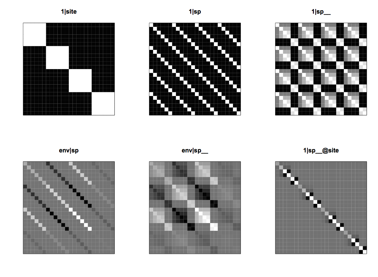
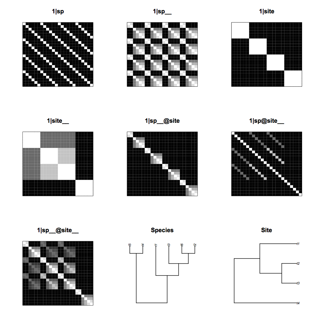
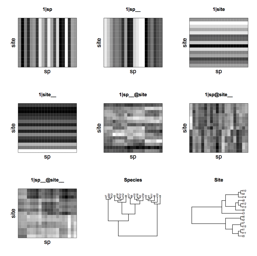
communityPGLMM() is a hierarchical mixed model that contains covariance matrices not only for the hierarchical structures in the data, but also phylogenies. The best way of explaining the model is with pictures, and the function communityPGLMM.plot.re() shows these. If show.image=T, it shows images of the covariance matrices for the random effects in the model, and if show.sim.image=T it gives a simulated example for each separate random effect. It also returns the covariance matrices in vcv and the simulated data in sim. For the figures in this chapter, I’ve used communityPGLMM.plot.re() to generate the matrices vcv and sim, and then plotted the matrices outside of communityPGLMM.plot.re(), because this allowed me to format the figures more appropriately for a book.
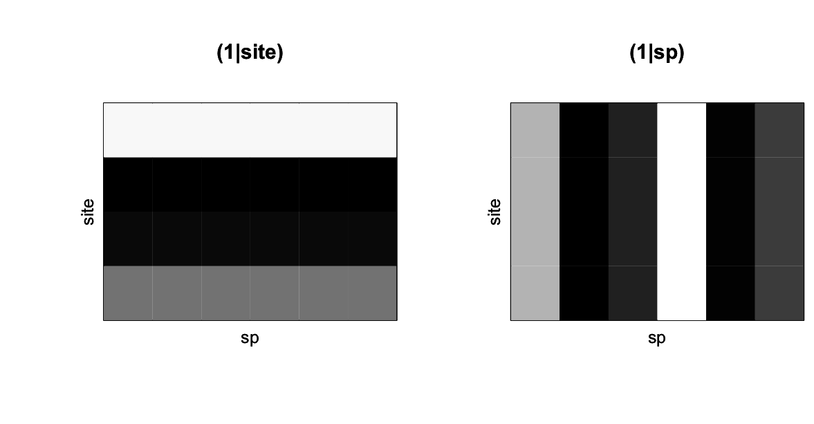
(1|site) and (1|sp) from communityPGLMM.plot.re() as would be produced with show.sim = T.Figure 4.1 shows the simulated abundances of six species among four sites, with whiter corresponding to higher values. The panel (1|site) gives the simulated mean abundances of species for each of the sites, and corresponds to the term (1|site) in the communityPGLMM() model. This term encapsulates the random effect that takes on a different value for each site. The panel (1|sp) gives a simulation of the random effect for species; each species is assigned at random a mean abundance across all sites. This term does not appear explicitly in the communityPGLMM() model, but it is there implicitly. In the model, the term (1|sp__) denotes a phylogenetic random effect for species, and when it is included, the non-phylogenetic effect (1|sp) is automatically included as well. In communityPGLMM() syntax, the double underscore __ denotes a phylogenetic random effect. Whenever a phylogenetic random effect is included, its corresponding non-phylogenetic random effect is included too. I’ll explain why a little later.
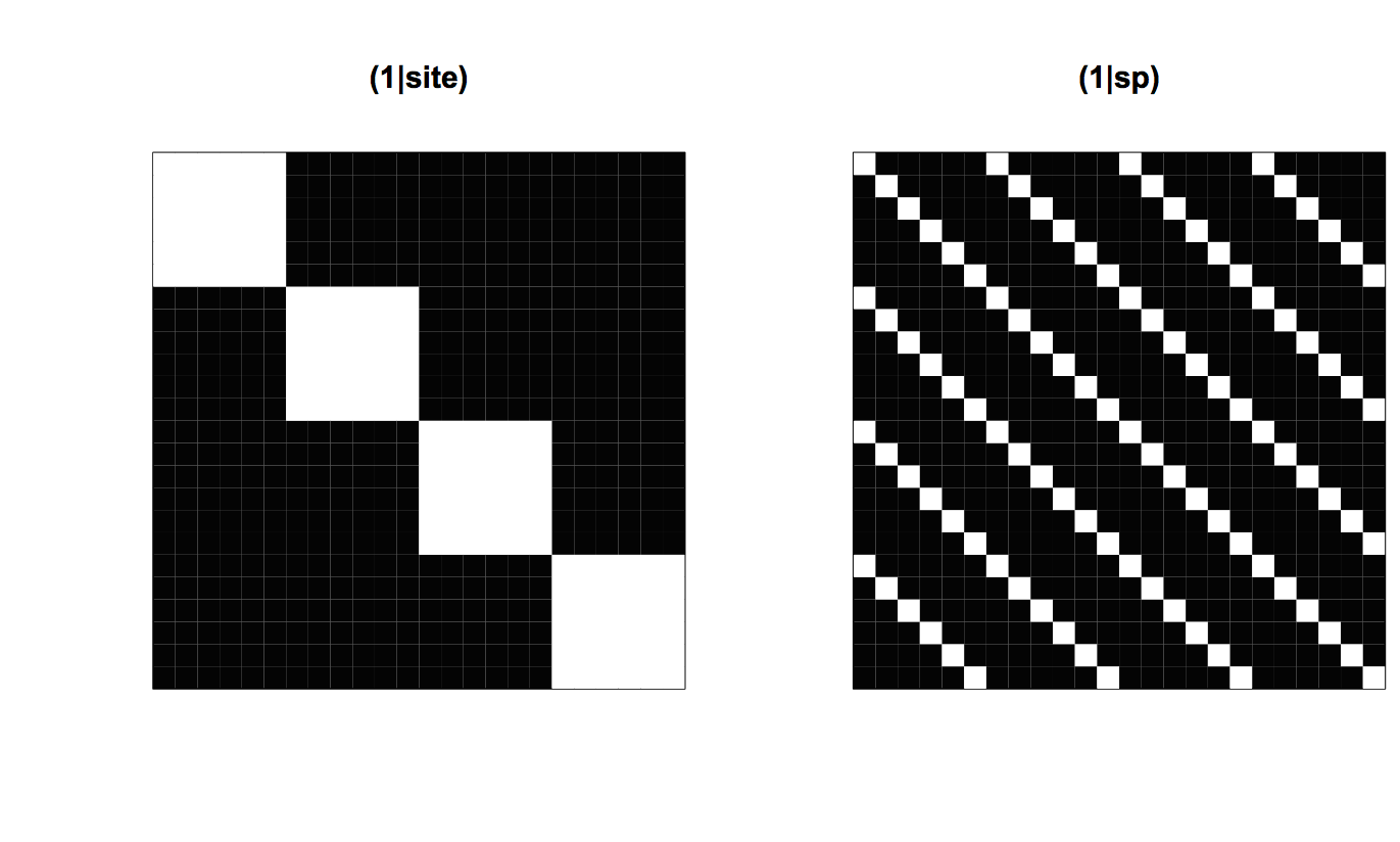
(1|site) and (1|sp) from communityPGLMM.plot.re() as would be produced with show.image = T.To see the structure of the model, it is necessary to look at the covariance matrices. Figure 4.2 shows the 24 x 24 element covariance matrices for (1|site) and (1|sp), with white showing high covariances. In fact, the covariances are either 1 or 0. The rows and columns of the covariance matrices are sorted so that species are nested within sites. Therefore, (1|site) has a block-diagonal form with 6 x 6 blocks of ones which correspond to the six species in the same site. (1|sp) contains 1s for each element corresponding to the same species in the 4 different sites. These covariance matrices are the same as typically found in mixed models that account for the hierarchical nature of the data.
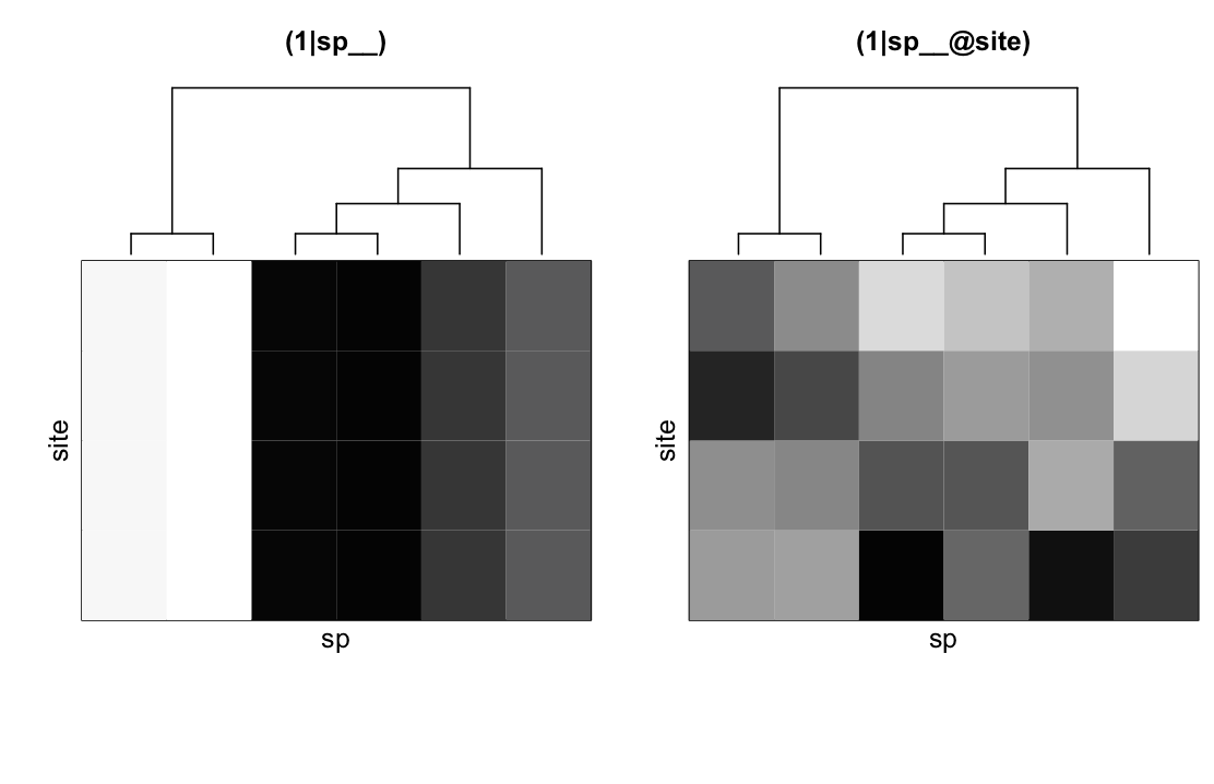
(1|sp__) and (1|sp__@site) from communityPGLMM.plot.re() as would be produced with show.sim = T.The two additional covariance matrices in the model give phylogenetic patterns in community composition. (1|sp__) gives the variation in mean abundance of species that has a phylogenetic signal (Fig. 4.3, left panel); this can be seen for the second and third species from the left that are phylogenetically closely related and have low mean abundances. (1|sp__@site) (Fig. 4.3, right panel) is phylogenetic attraction. Phylogenetically related species are more likely to occur in the same sites, although this is not due to their both having high overall abundances across all sites. Phylogenetic attraction just describes the case when related species are likely to both have low or both have high abundance in the same site. The two species on the left of (1|sp__@site) exemplify this pattern, with both being particularly (though randomly) low in the second site.
Phylogenetic attraction in the covariance matrix V in the simulation code is created using the Kronecker product of two matrices (the function kronecker()). This function takes the second matrix (in this case, Vphy) and replicates it according to the first matrix (the identity matrix with the number of diagonal elements equal to the number of sites). The function is clarified in the discussion of (1|sp__@site) that follows.
In the code for simulating the data, there is a line
# Standardize Vphy to have determinant = 1
Vphy <- Vphy/(det(Vphy)^(1/nspp))
This standardization is used to give a known value of the determinant of the covariance matrix regardless of the overall branch lengths of the input matrix phy. For example, a phylogeny might have branch lengths measured in genetic distance or millions of years of separation between species, and the value of branch lengths will be very different. The determinant measures the overall size or volume of a matrix, and therefore it gives a natural way to standardize matrices. The determinant is standardized to 1, because all identity matrices (for independent data) have determinants of 1. communityPGLMM() automatically performs this standardization, so that the values of the phylogenetic random effects (the phylogenetic variances) can be interpreted alongside the values of the non-phylogenetic random effects.
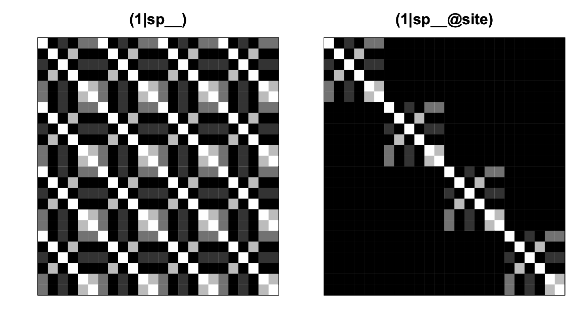
(1|sp__) and (1|sp__@site) from communityPGLMM.plot.re() as would be produced with show.image = T.The covariance matrices for (1|sp__) and (1|sp__@site) are given in figure 4.4, where like figure 4.2 species are nested within sites. The covariance matrix for (1|sp__) is densely populated: the covariance matrix for the phylogeny, Vphy, is tiled over the entire matrix. This occurs because (1|sp__) gives phylogenetic patterns in the mean abundance of species: if a species is common in one site, then a phylogenetically closely related species will likely have high abundance not only in this site, but also in any site. In contrast to (1|sp__), (1|sp__@site) gives phylogenetic attraction in which high abundance of a species in one site will only be associated with high abundance of a phylogenetically closely related species in the same site.
These comparisons among covariance matrices explain why inclusion of a phylogenetic random effect requires the inclusion of non-phylogenetic effects. For (1|sp__), the covariance between the same species in different sites is 1; this is also true of (1|sp), but for (1|sp) all other elements are 0. If (1|sp__) were included in a model without (1|sp), then any variation in mean abundance of species across all sites would potentially be picked up by (1|sp__) and might falsely be ascribed to phylogenetic signal. Including (1|sp) absorbs this species-specific variation so that tests of (1|sp__) only involve the phylogenetic covariances between species, rather than also the variances within species. Similarly, (1|sp__@site) has positive covariances in blocks along the diagonal of the covariance matrix, and so it has a similar structure to (1|site). If (1|site) were not included in the model, then any site-to-site variation in mean abundance of species might be ascribed to phylogenetic attraction. Even though (1|site) should most often be included in a model that contains (1|sp__@site), communityPGLMM() does not do this automatically, so you have to do it yourself. Unfortunately, including (1|sp) and (1|site) in the model increases the number of parameters that must be estimated, but they are necessary to prevent inflated type I errors in detecting phylogenetic patterns.
Finally, note that there are two phylogenetic patterns, one in the mean abundance of species and the other in the covariance in abundances of species in the same sites (phylogenetic attraction). These two phylogenetic patterns underscore the advantage of a modeling approach that can separate these two phylogenetic effects. It is difficult to derive a metric and permutation test for this pattern. The problem of different phylogenetic patterns multiplies when sites have their own phylogenies in bipartite data.
The output of communityPGLMM() is similar to lmer(), giving random effects and fixed effects. For this particular simulation, the estimates of all random effects were considerably larger than 0, including the two phylogenetic terms (1|sp__) and (1|sp__@site):
:Y ~ 1
logLik AIC BIC
-48.02 108.04 108.24
Random effects:
Variance Std.Dev
1|sp 0.1358 0.3685
1|sp__ 0.4695 0.6852
1|site 0.3238 0.5690
1|sp__@site 3.1830 1.7841
residual 0.1602 0.4002
Fixed effects:
Value Std.Error Zscore Pvalue
(Intercept) -0.03976 0.98530 -0.0404 0.9678
The P-values for the fixed effects can obtained from the Wald tests or LRTs, while P-values for the random effect can be obtained by LRTs. These are illustrated in the next subsection.
4.3.2 Type I errors and power
To investigate the ability of the PLMM to statistically identify phylogenetic attraction, I performed a simulation in which the strength of phylogenetic attraction was increased by increasing sd.attract, the parameter scaling the magnitude of the phylogenetic attraction covariance matrix. I then tested the null hypothesis that the estimate of sd.attract is zero with a LRT. I used two methods to determine the significance of the LRT: the standard chi-square approximation to the distribution of the deviance (twice the difference in log likelihoods between full and reduced models), and a bootstrapped distribution of the deviance under the H0. The code for these two tests is
<- communityPGLMM(Y ~ 1
+ (1|sp__)
+ (1|site)
+ (1|sp__@site),
data=d, tree=phy, REML=F)
mod.r <- communityPGLMM(Y ~ 1
+ (1|sp__)
+ (1|site),
data=d, tree=phy, REML=F)
dev <- 2*(mod.f$logLik - mod.r$logLik)
reject$LRT <- (pchisq(dev, df=1, lower.tail=F) < 0.05)
reject$boot0 <- (dev > LRT.crit)
The critical threshold value for the deviance in the bootstrap test, LRT.crit, is obtained by performing bootstrap simulations of the data using the following procedure, as was done for similar bootstrap tests in subsections 2.6.4 and 3.5.3:
- Using the estimated values of the reduce model with
sd.attract= 0 fit to the data, simulate a large number of datasets (e.g., 2000 for an alpha significance level of 0.05). - Refit both full (including
sd.attract) and reduced models to the simulated datasets, and calculate the LLRs and the corresponding deviances. -
LRT.critis the value which is exceeded by 0.05 of the bootstrapped values of the deviance.
Note that I’ve used ML for fitting the models, specifying REML=F; the default is REML=T. For performing a LRT on the covariance matrices, either ML or REML can be used for tests of random effects. When comparing fixed effects, though, only ML can be used, and therefore you should take care in which you are using. For this particular model, tests of the random effects using ML and REML give the same results.
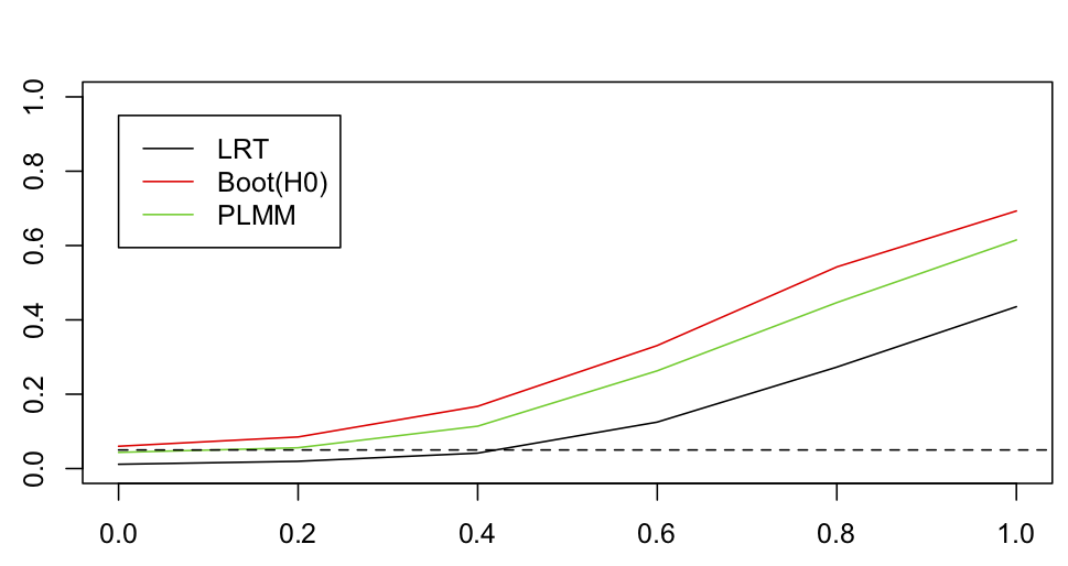
As shown in figure 4.5, the standard LRT with the chi-square approximation has deflated type I errors: only 0.023 of the simulated datasets were rejected. This implies that the P-values from the standard LRT are too high. The LRT with bootstrapped P-values under the null hypothesis H0 had correct type I errors and greater power than the standard LRT. Although it is always preferable to perform a bootstrap test under H0, for large datasets this becomes computationally challenging. Fitting a single simulated dataset with 50 species and 100 sites took 17 minutes on my old Macintosh, so a bootstrap with 2000 bootstrapped datasets would take 24 days. Because of the mathematics underlying the statistical analyses of communityPGLMM(), models that include nested terms like (1|sp__@site) run more slowly than models with only non-nested terms like (1|sp__). The standard LRT based on the chi-square approximation luckily has deflated rather than inflated type I errors. Therefore, if you use the standard LRT, it won’t give you P-values that are too low and increase you chances of falsely claiming a significant result. There is a moderate reduction in power, but this is far less serious than inflated type I errors.
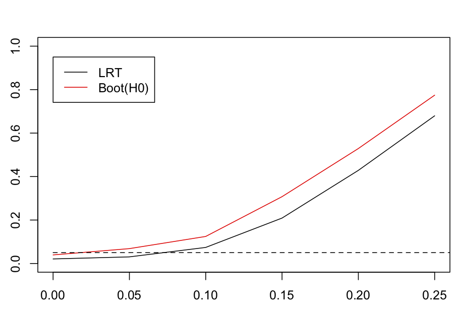
sd.attract = 0, 0.05, 0.1, 0.15, 0.2 and 0.25, the significance of sd.attract was tested with a standard LRT (LRT) and with a parametric bootstrap test of H0, Boot(H0).4.4 Phylogenetic repulsion
Phylogenetic repulsion is the opposite pattern from phylogenetic attraction, with phylogenetically related species less likely to have high abundance in the same site. Unlike phylogenetic attraction, when a phylogenetic covariance matrix generated under the assumption of Brownian motion evolution can be used to describe the possible positive covariances in species abundance, phylogenetic repulsion involves negative covariances in the abundances of related species. One way to derive a sensible covariance matrix for repulsion is to use the matrix inverse of the phylogenetic covariance matrix, V. The justification for this can be derived by assuming that species are competitors whose population dynamics follow a Lotka-Volterra competition model. If the competition coefficients that give the strength of competition between each pair of species are assumed to equal the elements of V, so that related species compete more with each other, then their relative abundances at equilibrium will be given by the inverse of V (Ives and Helmus 2011, appendix A).
A challenge in detecting phylogenetic repulsion is that phylogenetically related species may be more likely to occur in the same sites because they share values of a trait that make the site suitable for both of them (Helmus et al. 2007). Therefore, environmental differences among sites might obscure phylogenetic repulsion. This can be taken into account by including both phylogenetic repulsion and environmental factors in the same PLMM.
4.4.1 Phylogenetic repulsion PLMM
I simulated data with phylogenetic covariances in the mean abundance of species among sites. This was just to make the data look more realistic, since in real datasets there is generally large variation among the mean abundances of species. I selected a value for an environmental variable env from a normal distribution and assumed that the responses of species to env depend on an unmeasured trait trait; specifically, for species i and site j, the effect of env on abundance depends on trait(i) * env(j). The trait is phylogenetically correlated among species, giving the case in which related species respond to the environment in a similar way. Phylogenetic repulsion is incorporated using the inverse of the phylogenetic covariance matrix; the function solve() gives the inverse. After simulating the data, communityPGLMM() is used to fit them.
# Phylogenetic variation in mean species abundances
sd.sp <- 1
mean.sp <- rTraitCont(phy, model = "BM", sigma=sd.sp)
Y.sp <- rep(mean.sp, times=nsite)

# Site-specific environmental variation
sd.env <- 1
env <- rnorm(nsite, sd=sd.env)

# Phylogenetically correlated response of species to env
sd.trait <- 1
trait <- rTraitCont(phy, model = "BM", sigma=sd.trait)
trait <- rep(trait, times=nsite)

# Strength of phylogenetic repulsion
sd.repulse <- 1
Vphy <- vcv(phy)

# Standardize Vphy to have determinant = 1
Vphy <- Vphy/(det(Vphy)^(1/nspp))
V.repulse <- kronecker(diag(nrow=nsite, ncol=nsite), solve(Vphy))
Y.repulse <- array(t(rmvnorm(n=1, sigma=sd.repulse^2*V.repulse)))

# Residual error
sd.e <- 1
Y.e <- rnorm(nspp*nsite, sd=sd.e)

# Construct the dataset
d <- data.frame(sp=rep(phy$tip.label, times=nsite),
	site=rep(1:nsite, each=nspp), env=rep(env, each=nspp))

# Simulate abundance data
d$Y <- Y.sp + Y.repulse + trait * d$env + Y.e

# Analyze the model
summary(communityPGLMM(Y ~ 1
	+ env
	+ (1|site)
	+ (1|sp__)
	+ (env|sp__)
	+ (1|sp__@site),
	repulsion=T, data=d, tree=phy))

logLik    AIC    BIC
-39.54  97.08  97.38

Random effects:
             Variance   Std.Dev
1|site      5.423e-07 0.0007364
1|sp        1.080e+00 1.0391595
1|sp__      7.798e-01 0.8830389
env|sp      1.000e-01 0.3162366
env|sp__    8.627e-01 0.9288251
1|sp__@site 1.814e-01 0.4259167
residual    4.016e-01 0.6337248

Fixed effects:
                Value Std.Error  Zscore Pvalue
(Intercept) -0.017754  0.902921 -0.0197 0.9843
env         -0.159704  0.833823 -0.1915 0.8481
In the communityPGLMM() model output, (1|site) gives the variation among sites in the mean abundance of species they contain, (1|sp) and (1|sp__) give non-phylogenetic and phylogenetic variation in mean species abundances, (env|sp) and (env|sp__) give the non-phylogenetic and phylogenetic response of species to env, and (1|sp__@site) gives phylogenetic repulsion. The nested random effect (1|sp__@site) is specified as giving repulsion rather than attraction by the statement repulsion=T. The covariance matrices for the model are depicted in figure 4.6 using communityPGLMM.plot.re() to generate covariance matrices. The three covariance matrices (1|site), (1|sp) and (1|sp__), are comparable to those in the model for phylogenetic attraction (Figs. 4.2 and 4.4), while (env|sp), (env|sp__), and (1|sp__@site) require explanation.
(1|site) gives the variation among sites in the mean abundance of species they contain, (1|sp) and (1|sp__) give non-phylogenetic and phylogenetic variation in mean species abundances, (env|sp) and (env|sp__) give the non-phylogenetic and phylogenetic responses of species to env, and (1|sp__@site) gives phylogenetic repulsion.Explaining (env|sp) requires computing the covariances in species abundances caused by their response to the environmental factor env. This is given by the product trait(i) * env(k) for species i in site k. The response of species i to env, trait(i), is a random variable, while env(k) is a fixed value known for site k. Therefore, the variance in trait(i) * env(k) is
env(k)2 * var[trait(i)].
In words, the variance in the abundance of species i in site k scales with the square of the value of the environmental factor in site k. This makes intuitive sense, because if the response of species to env is a random variable, and all you know is that the value of env in a site is very large, then you would be very uncertain about whether species i would have very high or very low abundance. The values of env for the four sites in the simulated example are -1.63, 2.25, -0.96, and -0.83. Therefore, site 2 has the highest variance, and site 4 has the lowest.
The same reasoning explains the pattern of covariances in the abundance of species i between sites given by (env|sp). For sites k and l, these are
env(k) * env(l) * var[trait(i)].
If env(k) and env(l) have opposite sign, then there will be negative covariances between the abundances of species i in sites k and l. This is the case for sites 1 and 2, for example. This makes intuitive sense, because if you know that sites 1 and 2 differ in env but you don’t know whether species i responds positively or negatively, you still know that species i is likely to have different abundances between sites 1 and 2. Although this structure of the random effect (env|sp) might seem unfamiliar, it is exactly how random effects for slopes are operating in all mixed models (see, for example, the lme4 documentation).
The random effect (env|sp__) is similar to (env|sp), although it also incorporates phylogenetic covariances in the values of trait(i) and trait(j) for species i and j. For the general case of species i and j, and sites k and l, the covariance is
env(k) * env(l) * cov[trait(i), trait(j)].
This is shown in the (env|sp__) matrix in figure 4.6.
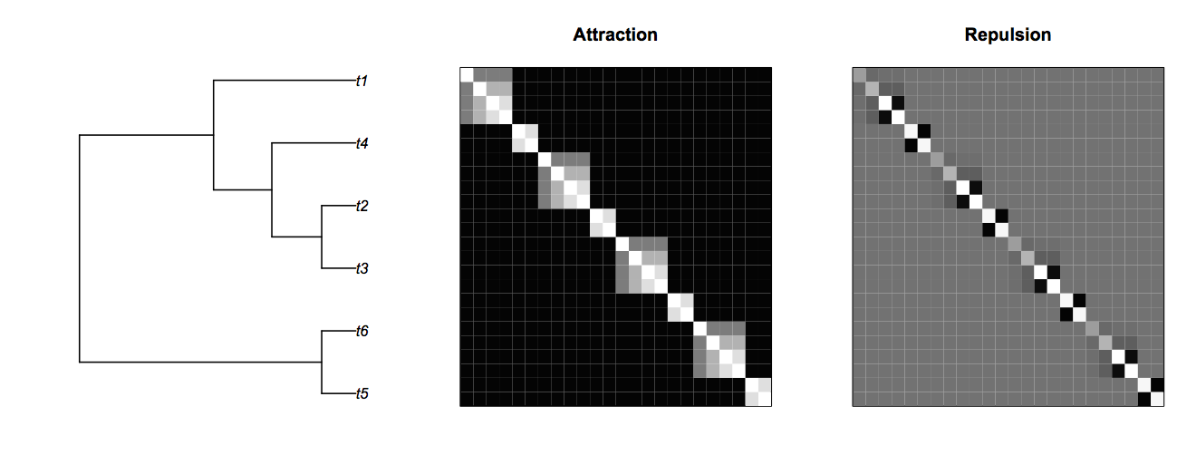
Finally, the phylogenetic repulsion covariance matrix (1|sp__@site) can be best understood in comparison to the phylogenetic attract matrix (Fig. 4.7). Here, species that are closely related, for example species t5 and t6 (species 5 and 6 within each site) are likely to show high phylogenetic attraction given by the covariance matrix V. However, in the phylogenetic repulsion matrix given by the inverse of V, species t5 and t6 have negative covariances. The “background” color of the repulsion covariance matrix is gray, rather than black as in the attraction covariance matrix, only because the repulsion covariance matrix has negative elements; the background covariances for species between different sites are zero in both matrices.
The statistical challenge of detecting phylogenetic repulsion when phylogenetically related species respond similarly to an environmental factor can be shown by comparing the covariance matrices (env|sp__) and (1|sp__@site) (Fig. 4.8). The phylogenetic repulsion matrix (1|sp__@site) is the inverse of the phylogenetic attraction matrix, and the phylogenetic attraction matrix appears in blocks along the diagonal of (env|sp__) multiplied by env2. This means that the phylogenetic effects within sites in part cancel each other out, which is seen by taking the sum of (env|sp__) and (1|sp__@site) (Fig. 4.8). This acts to mask the effect of phylogenetic repulsion.
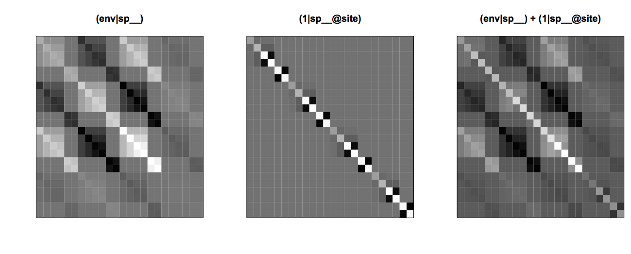
(env|sp__), phylogenetic repulsion (1|sp__@site), and the combined effects of the environmental factor and phylogenetic repulsion.4.4.2. Testing for phylogenetic repulsion
A test for phylogenetic repulsion can be performed with a LRT comparing the communityPGLMM() models with and without (1|sp__@site).
<- communityPGLMM(Y ~ 1
+ env
+ (1|site)
+ (1|sp__)
+ (1|sp__@site)
+ (env|sp__),
data=d, repulsion=T, tree=phy, REML=T)
summary(mod.f)
mod.r <- communityPGLMM(Y ~ 1
+ env
+ (1|site)
+ (1|sp__)
+ (env|sp__),
data=d, repulsion=T, tree=phy, REML=T)
pchisq(2*(mod.f$logLik - mod.r$logLik), df=1, lower.tail=F)
For the case of 20 species and 15 sites, even relatively weak phylogenetic repulsion (sd.repulse <- 0.5) is generally identified as highly significant. For a specific simulation, the LRT test gave P = 0.007. To see how phylogenetically correlated species-specific responses to env can obscure phylogenetic repulsion, I fit the same simulated example without env:
<- communityPGLMM(Y ~ 1
+ (1|site)
+ (1|sp__)
+ (1|sp__@site),
data=d, repulsion=T, tree=phy, REML=T)
summary(mod.f)
mod.r <- communityPGLMM(Y ~ 1
+ (1|site)
+ (1|sp__),
data=d, repulsion=T, tree=phy, REML=T)
pchisq(2*(mod.f$logLik - mod.r$logLik), df=1, lower.tail=F)
In this case, the LRT gave P = 0.21, so no phylogenetic repulsion was detected. The huge improvement in detecting phylogenetic signal by including env doesn’t always happen, but it is more likely than not; you can use the R code to simulate more examples.
I have used the standard LRT with the chi-square approximation in this example, although it is possible to perform a parametric bootstrap LRT under H0 of no phylogenetic repulsion. However, because I know that the LRT is conservative from section 4.3 (and from other simulations) and gives P-values that are if anything too high, and because I’m not worried about power, I’ve only used the time-saving standard LRT.
4.5 Can traits explain phylogenetic patterns?
If phylogenetic correlations among species trait values are responsible for phylogenetic attraction of species among sites, then incorporating information about these traits into a PLMM should remove any phylogenetic attraction. This intuitive conclusion was largely supported by analyses of two real datasets by Li et al. (2017). For the dataset with the greatest information about trait values, we showed that including these values in a PLMM explained all of the phylogenetic attraction in the data. For the second dataset, trait values explained most but not all of the phylogenetic signal, although in the second dataset the number of traits available was limited.
To show how trait information can explain phylogenetic attraction, I simulated data using three traits that determine the response of species to three environmental variables that are distributed independently among sites. Although the data are simulated knowing information about environmental variables among sites, I assume that environmental information is not available when analyzing the data.
<- rep(rnorm(nsite, sd=sd.env), each=nspp)
env2 <- rep(rnorm(nsite, sd=sd.env), each=nspp)
env3 <- rep(rnorm(nsite, sd=sd.env), each=nspp)
trait1 <- rTraitCont(phy, model = "BM", sigma = sd.trait)
trait2 <- rTraitCont(phy, model = "BM", sigma = sd.trait)
trait3 <- rTraitCont(phy, model = "BM", sigma = sd.trait)
Y.e <- rnorm(nspp*nsite, sd=sd.e)
d <- data.frame(sp=rep(phy$tip.label, times=nsite),
site=rep(1:nsite, each=nspp),
trait1=rep(trait1, times=nsite),
trait2=rep(trait2, times=nsite),
trait3=rep(trait3, times=nsite))
d$Y <- b0 + c1*env1 + c2*env2 + c3*env3
+ f1*d$trait1*env1 + f2*d$trait2*env2 + f3*d$trait3*env3
+ Y.e
In the simulation of species abundances Y, c1*env1 makes the mean abundance of species in a given site depend on the value of env1 in that site, with the coefficient c1 determining the strength of this affect. The term f1*d$trait1*env1 gives the species-specific response to env1 that depends on the value of trait1, scaled by the coefficient f1. Thus, f1*d$trait1 can be thought of the slope of species abundances with respect to env1, with each species having a different slope depending on their value of trait1.
I fit the simulated data using two models: the model for phylogenetic attraction presented in section 4.3, and a model that includes the trait information available for the species.
# Fitting model without trait information
mod.trait0.f <- communityPGLMM(Y ~ 1
	+ (1|sp__)
	+ (1|site)
	+ (1|sp__@site),
	tree=phy, data=d)
mod.trait0.r <- communityPGLMM(Y ~ 1
	+ (1|sp__)
	+ (1|site),
	tree=phy, data=d)
summary(mod.trait0.f)
pvalue <- pchisq(2*(mod.trait0.f$logLik - mod.trait0.r$logLik),
	df=1, lower.tail=F)

# Fitting model with trait information
mod.trait123.f <- communityPGLMM(Y ~ 1
	+ trait1
	+ trait2
	+ trait3
	+ (trait1|site)
	+ (trait2|site)
	+ (trait3|site)
	+ (1|sp__)
	+ (1|site)
	+ (1|sp__@site),
	tree=phy, data=d)
mod.trait123.r <- communityPGLMM(Y ~ 1
	+ trait1
	+ trait2
	+ trait3
	+ (trait1|site)
	+ (trait2|site)
	+ (trait3|site)
	+ (1|sp__)
	+ (1|site),
	tree=phy, data=d)
summary(mod.trait123.f)
pvalue <- pchisq(2*(mod.trait123.f$logLik - mod.trait123.r$logLik),
	df=1, lower.tail=F)
The first model for phylogenetic attraction has terms (1|sp__) to account for non-phylogenetic and phylogenetic variation in mean species abundances, (1|site) to account for differences in mean species abundances among sites, and (1|sp__@site) for phylogenetic attraction. The second model has the same terms plus terms (trait|site) for each trait. These terms imply that each site may favor species with different values of trait. If the value of env were known for each site, then it would be possible to include a trait-by-environment interaction trait:env as a fixed effect in the model; this term was used in the simulation to generate phylogenetic responses of species to environmental factors. However, since we assume that env is not known in the dataset, the model specifies only that sites differ in some unknown way that selects differently for species depending on their value of trait. I also included fixed effects for each trait, since traits are also included as slopes in the random effect (trait|site). The reason to include trait fixed effects is that they give the mean effect of trait for each species and serve the same role as a main effect in a regression model that includes interaction terms: if interaction terms are in a model, so too should be the corresponding main effects for each term in the interaction.
For both models I tested the significance of phylogenetic signal given by (1|sp__@site) using a standard LRT. The results of the fits show that incorporating trait information explains the phylogenetic attraction.
summary(mod.trait0.f)

logLik    AIC    BIC
-512.8 1037.7 1053.0

Random effects:
             Variance   Std.Dev
1|sp        1.248e-02 0.1117275
1|sp__      3.652e-07 0.0006043
1|site      1.857e+00 1.3626107
1|sp__@site 2.921e-01 0.5404801
residual    1.020e+00 1.0099133

pvalue
[1] 3.672444e-16

summary(mod.trait123.f)

logLik    AIC    BIC
-472.8  969.6 1000.3

Random effects:
             Variance   Std.Dev
trait1|site 4.597e-01 0.6780417
trait2|site 2.934e-07 0.0005417
trait3|site 1.625e-01 0.4031411
1|sp        2.510e-02 0.1584391
1|sp__      2.301e-07 0.0004797
1|site      2.530e+00 1.5905141
1|sp__@site 3.918e-06 0.0019795
residual    9.759e-01 0.9878592

pvalue
[1] 0.8820785
In the first model without trait values, the random effect (1|sp__@site) is highly significant (P < 10^-15), while in the second model it is not (P = 0.88). Thus, the trait values in the second model absorbed the variation that was attributed to phylogenetic attraction in the first model. This is only a single simulated example, but you can use the code to see that this is a common result. Also, note that the P-value for (1|sp__@site) differed so much between models, I was not very concerned about the possible loss of power by not performing a bootstrap LRT under H0.
The consequences of adding trait information on phylogenetic attraction can be seen by investigating the covariance matrices and comparing them to the trait data. A simulation for six species and four sites produced the dataset:
Covariance matrices for this dataset are given in figure 4.9. Each of the covariance matrices for the trait random effects (trait|site) contains the phylogenetic covariances among species, but they vary in their weightings. For example, species t3 (the second species in each site) has the highest value of trait1 and therefore has the highest variance in the covariance matrix (trait1|site). Species t3 is related to t2 and t4 (taking positions 2, 1, and 3 in each community), so there are phylogenetic covariances between these species seen as 3 x 3 blocks of nine cells in the covariance matrix. Because the values of trait1 are low for the other three species (taking positions 4, 5, and 6), they don’t exhibit strong positive covariances. Covariance matrices (trait2|site) and (trait3|site) similarly have phylogenetic covariances, but weighted differently from (trait1|site) due to the different distribution of trait values among species. The sum of (trait1|site), (trait2|site) and (trait3|site) averages over the specific weights of species, and the resulting covariance matrix is similar to the matrix (1|sp__@site) giving phylogenetic attraction. This explains why, in the model with trait values analyzed above, there is little phylogenetic attraction detected; the phylogenetic covariance in species abundances within sites is accounted for by the combined random effects of traits within sites.
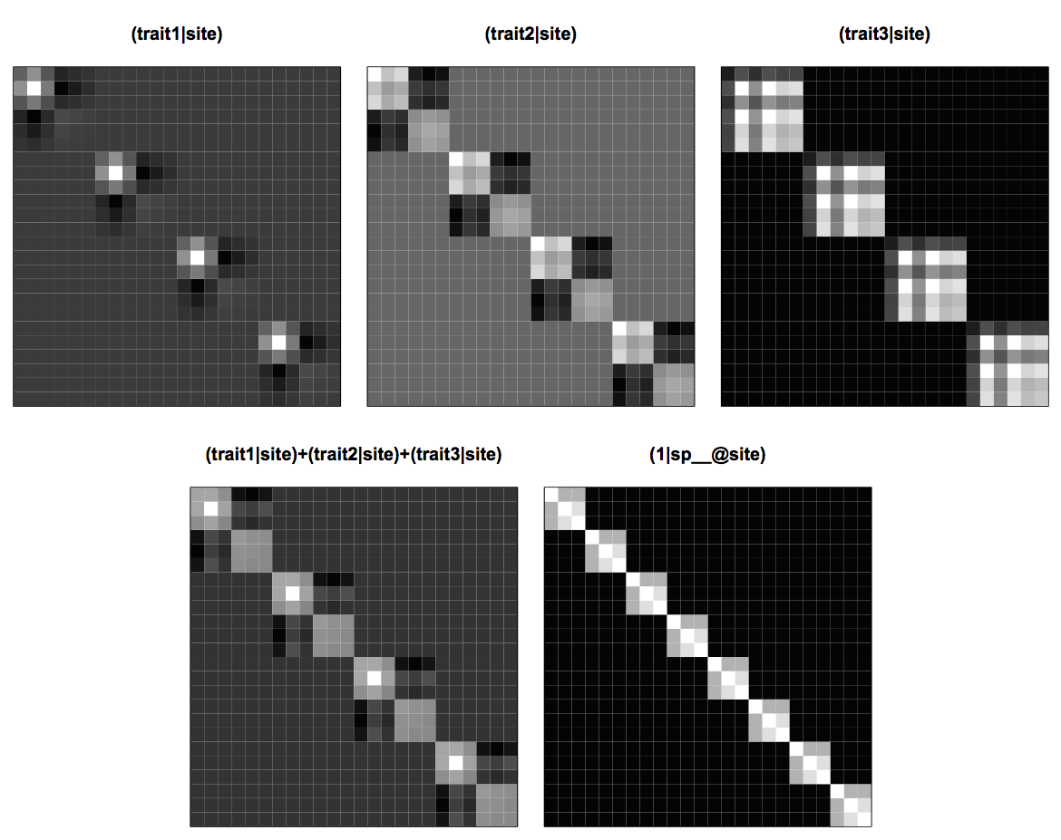
(trait1|site), (trait2|site) and (trait3|site), the sum of all three of these matrices, and the phylogenetic attraction matrix (1|sp__@site).It is not necessary to have information on all trait values for traits to absorb some of the phylogenetic attraction in the model. In other words, even information on just a single trait might absorb a lot of the phylogenetic attraction that is observed without information about this trait. I’ve left you to explore this as an exercise.
4.6 Trait-by-environment interactions
In searching for phylogenetic repulsion (section 4.4), I assumed information was available for environmental factors, and in asking for explanations of phylogenetic attraction (section 4.5), I assumed trait information was available. If both trait and environmental information are available, then it should be possible to explain all patterns in the data without the need for a phylogeny. This assumes, however, that all traits and environmental factors are known. If they are not, then unknown traits and environmental factors can produce correlations in the data. Ignoring these correlations is like ignoring hierarchical correlations (Chapter 2) or phylogenetic correlations in comparisons among species (Chapter 3): inflated type I errors and low power.
To illustrate these issues, I’ll set up and analyzed the problem investigated by Li and Ives (2017). Assume that there are two traits, trait1 and trait2, and two environmental factors env1 and env2. Values of trait1 and env1 are known, while trait2 and env2 are unknown. The mean abundances of species across sites depend on both traits, and the mean abundances of species within sites depend on both environmental factors. Finally, both trait1 and trait2 affect the response of species to env1. The reason for having trait2 affect species responses to env1 is to generate phylogenetic signal in species responses to env1 that is not due to trait1. This situation is likely in real systems, since multiple traits are generally involved in species adaptations to environmental factors, and it is often likely that some of these traits are unknown. The code to simulate the data is
<- 20
nsite <- 15
# Simulate a phylogenetic tree
phy <- compute.brlen(rtree(n = nspp), method = "Grafen", power = 1)
# Generate two environmental variables that are randomly distributed
# among sites. Only values of env1 are known in the dataset.
sd.env <- 1
env1 <- rnorm(nsite, sd=sd.env)
env2 <- rnorm(nsite, sd=sd.env)
env2 <- rep(env2, each=nspp)
# Generate two traits that differ phylogenetically among species.
# Both traits govern the response of species to env1,
# but only the values of trait1 are known in the dataset.
sd.trait <- 1
trait1 <- rTraitCont(phy, model = "BM", sigma = sd.trait)
trait2 <- rTraitCont(phy, model = "BM", sigma = sd.trait)
trait2 <- rep(trait2, times=nsite)
# Simulate a dataset. The terms 'f11*d$trait1*env1' and 'f21*d$trait2*env1'
# give the trait-by-environment interactions.
b0 <- 0
b1 <- 1
b2 <- 1
c1 <- 1
c2 <- 1
f11 <- .5
f21 <- .5
sd.e <- 1
Y.e <- rnorm(nspp*nsite, sd=sd.e)
d <- data.frame(sp=rep(phy$tip.label, times=nsite),
site=rep(1:nsite, each=nspp), trait1=rep(trait1,
times=nsite), env1=rep(env1, each=nspp))
d$Y <- b0 + b1*d$trait1 + b2*trait2 + c1*d$env1
+ c2*env2 + f11*d$trait1*d$env1 + f21*trait2*d$env1
+ Y.e
The statistical question is whether the trait-by-environment interaction trait1:env1 is different from zero, which corresponds to the coefficient f11 in the simulation. The statistical challenge is that there is phylogenetic signal in the data. Specifically, we know from the simulations used to produce the data that there is phylogenetic signal in the response of species to env1 that is not due to trait1. This can be included in the model with a term (env1|sp__) which corresponds to f21*trait2*d$env1 in the simulation. Similarly, there is also phylogenetic signal in the mean abundances of species caused by trait2 which can be included in the model with (1|sp__); this corresponds to b2*trait2 in the simulation. If phylogenetic signal is not included, then the corresponding terms are (env1|sp) and (1|sp). Thus, the two models needed to see the effects of incorporating phylogenetic signal on the statistical ability to detect the trait-by-environment interaction trait1:env1 are
<- communityPGLMM(Y ~ 1
+ trait1*env1
+ (1|sp__)
+ (1|site)
+ (env1|sp__),
tree=phy, data=d)
summary(mod.f)
mod.0 <- communityPGLMM(Y ~ 1
+ trait1*env1
+ (1|sp)
+ (1|site)
+ (env1|sp),
tree=phy, data=d)
summary(mod.0)
Note that the second model is just a non-phylogenetic LMM that accounts for the hierarchical structure of the data but not phylogenetic correlations. Therefore, it could be fit with lmer() from the package lme4.
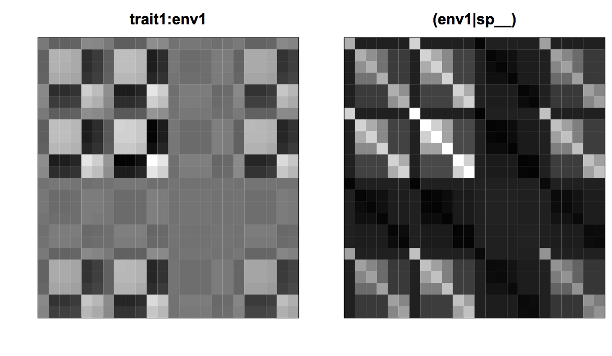
The phylogenetic covariances are expected to create problems for type I errors and/or statistical power. These problems can be anticipated by comparing the effect of the interaction term trait1:env1 on species abundances with the covariance matrix for (env1|sp__). The left panel of figure 4.10 gives the squared errors in species abundances that are attributable to the trait1:env1 interaction; each element in the matrix gives the product of trait1(i) * trait1(j) * env1(k) * env1(l) for species i and j, and sites k and l. These are thus the fixed effects equivalent to the covariance matrix for the random effects. The similarity between the matrix for trait1:env1 and (env1|sp__) shows that statistically it will be difficult to distinguish the effect of the trait1:env1 interaction from phylogenetic signal in the effect of env1 that occurs in the covariances of the residual variation. This likely leads to the two problems found for phylogenetic analyses in section 3.6.2 (Fig. 3.9). First, for the correctly specified model with (env1|sp__), this will likely lead to a decrease in power to detect a significant trait1:env1 interaction compared to the case when there were no phylogenetic signal in the effect of env1. Second, for the mis-specified model that ignores the phylogenetic signal in the effect of env1, the true phylogenetic signal from env1 will falsely be attributed to the trait1:env1 interaction and hence lead to inflated type I errors when there is phylogenetic signal in trait1.
trait1:env1 on the squared residuals and the covariance matrix for (env1|spp__).I tested these anticipated problems with type I errors and power for the non-phylogenetic LMM as done in Li and Ives (2017). I generated power curves for the cases in which trait1 either didn’t or did have phylogenetic signal. These correspond to the cases presented for phylogenetic comparative methods in which power curves for a regression coefficient were generated when the associated x variable either didn’t or did have phylogenetic signal (section 3.6.2, Fig. 3.9). Failing to account for phylogenetic signal using the term (env1|sp__) had the anticipated effects. First, when there was no phylogenetic signal in trait1, the LMM that did not include the phylogeny had poor statistical power (Fig. 4.11, left panel). Second, when there was phylogenetic signal in trait1, the LMM that did not include the phylogeny had inflated type I errors (Fig. 4.11, right panel).
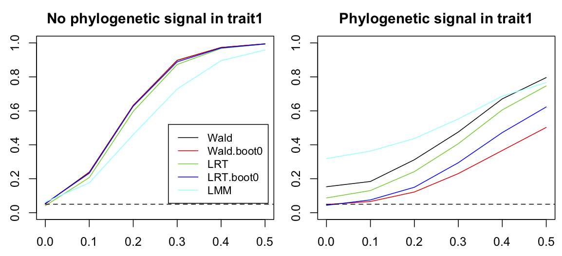
trait1:env1 interaction in a PLMM. Datasets of 20 species distributed among 15 sites were simulated assuming that trait1 didn’t (left panel) or did (right panel) have phylogenetic signal. For each level of f11 = 0, 0.2, 0.4, 0.6, 0.8 and 1.0, 2000 simulations were performed and the rejection rates calculated for communityPGLMM() using a Wald test, a Wald test bootstrapped under H0, a LRT test, and a LRT test bootstrapped under H0. Finally, a non-phylogenetic LMM was fit to the data. The other parameters used to simulate the data are b0 = 0, b1 = 1, b2 = 1, c1 = 1, c2 = 1, f21 = 0.5, sd.env = 1, sd.trait = 1, and sd.e = 1.In addition to showing the importance of including phylogenetic information, figure 4.11 also compares different methods for computing P-values for regression coefficients in the PLMM. P-values can be computed by either Wald tests or LRTs, and I also performed both tests by bootstrapping the distributions of Z scores (Wald test) and LLRs (LRT). When there is no phylogenetic signal in trait1, all methods had good type I errors and almost identical power. However, when there was phylogenetic signal in trait1, the Wald test and LRT both had inflated type I errors, especially the Wald test (although not as bad as the LMM). As should be the case, the parametric bootstrap tests around H0 had correct type I errors, and the bootstrapped LRT had slightly greater power. The inflated type I errors for the non-bootstrap tests means that a parametric bootstrap should be performed.
4.7 Bipartite phylogenetic patterns
So far we have assumed that only species have phylogenetic patterns in their distributions among sites. For problems such as the association between pollinators and plants, or disease and hosts, the sites used by pollinators or diseases have a phylogeny as well. For example, closely related pollinator species might be more likely to feed from phylogenetically related plant species, or two closely related host species might be more susceptible to the same disease. Adding a phylogeny for the site introduces nothing new statistically, although it does add more patterns to understand and analyze.
In this section, I’ll first illustrate the problem of identifying phylogenetic attraction for both species and sites. I’ll then ask whether phylogenetic attraction among sites (closely related sites being more likely to be associated with closely related species) can be statistically attributed to trait differences among sites. Both scenarios are motived by the study in Rafferty and Ives (2013) that investigated the patterns of association of pollinator visits to plants, and whether visitation patterns among plants were explained by similarities among their trait values. I’ll continue to use “sites” for one of the groups of species in the bipartite data; this makes it easier to integrate the discussion into the rest of the chapter. But throughout I’ll assume that species are pollinators, sites are plants, trait refers to pollinator traits, and env refers to plant traits.
4.7.1 Phylogenetic attraction for species and sites
A simulation for the distribution of species among sites including phylogenetic attraction for both species and sites is
# Simulate species means
mean.sp <- rTraitCont(phy.sp, model = "BM", sigma=1)
# Replicate values of mean.sp over sites
Y.sp <- rep(mean.sp, times=nsite)

# Simulate site means
mean.site <- rTraitCont(phy.site, model = "BM", sigma=1)
# Replicate values of mean.site over sp
Y.site <- rep(mean.site, each=nspp)

# Generate covariance matrix for phylogenetic attraction among species
sd.sp.attract <- 1
Vphy.sp <- vcv(phy.sp)
Vphy.sp <- Vphy.sp/(det(Vphy.sp)^(1/nspp))
V.sp <- kronecker(diag(nrow=nsite, ncol=nsite), Vphy.sp)
Y.sp.attract <- array(t(rmvnorm(n=1, sigma=sd.sp.attract^2*V.sp)))

# Generate covariance matrix for phylogenetic attraction among sites
sd.site.attract <- 1
Vphy.site <- vcv(phy.site)
Vphy.site <- Vphy.site/(det(Vphy.site)^(1/nsite))
V.site <- kronecker(Vphy.site, diag(nrow=nspp, ncol=nspp))
Y.site.attract <- array(t(rmvnorm(n=1, sigma=sd.site.attract^2*V.site)))

# Generate covariance matrix for phylogenetic attraction of species:site interaction
sd.sp.site.attract <- 1
V.sp.site <- kronecker(Vphy.site, Vphy.sp)
Y.sp.site.attract <- array(t(rmvnorm(n=1, sigma=sd.sp.site.attract^2*V.sp.site)))

# Simulate residual error
sd.e <- 0.5
Y.e <- rnorm(nspp*nsite, sd=sd.e)

# Construct the dataset
d <- data.frame(sp=rep(phy.sp$tip.label, times=nsite),
	site=rep(phy.site$tip.label, each=nspp))

# Simulate abundance data
d$Y <- Y.sp + Y.site + Y.sp.attract + Y.site.attract + Y.sp.site.attract + Y.e
The code first simulates mean species abundances from the species phylogeny, phy.sp, and the mean abundance of species in each site from the site phylogeny, phy.site. These are expanded to the site-species data points and saved in the arrays Y.sp and Y.site. The code then creates the phylogenetic covariance matrices for phylogenetic attraction for species, sites, and the species-site interaction, Vphy.sp, Vphy.site, and V.sp.site; I’ll show the structure of these matrices below. From these covariance matrices, site-species data points are generated and saved in the arrays Y.sp.attract, Y.site.attract, and Y.sp.site.attract. Finally, random error is generated, and all arrays are added together to make the simulated dataset.
The covariance matrices can be visualized using communityPGLMM.plot.re(). Figure 4.12 shows the covariance matrices for the case of six species (pollinators) and four sites (plants). Phylogenetic attraction for species is the same as shown previously in figure 4.3: closely related species are more likely to have high or low abundances within the same site as given by (1|sp__@site). Phylogenetic attraction has the same structure for the sites: closely related sites are more likely to contain high or low abundances of the same species as given by (1|sp@site__). The new phylogenetic attraction covariance matrix, (1|sp__@site__), describes the pattern in which closely related species are more likely to occur in closely related sites. This is produced by tiling the species covariance matrix (seen in (1|sp__@site)) across the site-species covariance matrix, with each tile weighted by the site covariance matrix (seen in (1|site__)).
communityPGLMM.plot.re(). The figure also shows the species and site phylogenies.Another way to visualize the covariance structure of the model is to simulate data from the covariance matrices using communityPGLMM.plot.re(); figure 4.13 shows an example with 20 species and 15 sites. The phylogenetic attraction of species within sites, (1|sp__@site), generates sections of rows corresponding to related species that are all high or low, showing related species having either high or low abundances within the same site. Similarly, the phylogenetic attraction of sites to contain the same species, (1|sp@site__), generates sections of columns corresponding to the same species that have high or low abundance in related sites. Finally, (1|sp__@site__) contains blocks in which related species in related sites have high or low abundances.
communityPGLMM.plot.re(). The figure also shows the species and site phylogenies.These simulated data can be fit by including all seven random effects in communityPGLMM(). Statistical tests for significance of the random effects are performed with LRTs. Because there are seven random effects, there may be problems with finding the true ML or REML parameter values for the random effects. Random effects are numerically challenging, because they have a boundary at zero. Therefore, the optimizer used to find the parameter values that give the highest likelihoods might have to walk up along this zero boundary, and most optimizers have a difficult time doing this. Therefore, it is worth using a few tricks. One is to add random effects one at a time, and use the estimated random effects terms from each model as starting values for the following model. For the LRT, I started with the reduced model and added the random effect that is the subject of the statistical test, in this case (1|sp__@site__). To fit the full model, I used the variances of the random effects terms estimated by the reduced model c(mod.r$ss, .01)^2 as the starting values for s2.init in the full model, with the value of s2.init for (1|sp__@site__) that is not in the reduced model set to 0.012.
<- communityPGLMM(Y ~ 1
+ (1|sp__)
+ (1|site__)
+ (1|sp__@site)
+ (1|sp@site__),
data=d, tree=phy.sp, tree_site=phy.site)
mod.f <- communityPGLMM(Y ~ 1
+ (1|sp__)
+ (1|site__)
+ (1|sp__@site)
+ (1|sp@site__)
+ (1|sp__@site__),
data=d, tree=phy.sp, tree_site=phy.site, s2.init=c(mod.r$ss, .01)^2)
pvalue <- pchisq(2*(mod.f$logLik - mod.r$logLik), df=1, lower.tail=F)
An example for this analysis for a simulated dataset is
-699.6 1417.2 1440.3
Random effects:
Variance Std.Dev
1|sp 0.001954 0.0442
1|sp__ 0.062437 0.2499
1|site 0.816100 0.9034
1|site__ 2.628756 1.6213
1|sp__@site 0.664351 0.8151
1|sp@site__ 1.423309 1.1930
1|sp__@site__ 1.308493 1.1439
residual 0.131048 0.3620
pvalue
[1] 2.554821e-08
In this simulation, the P-value for (1|sp__@site__) from the LRT was very low, implying a strong interaction between the species and site phylogenies: phylogenetically related species were more likely to have high abundances in phylogenetically related sites. Because the P-value is so low, I felt safe not performing a parametric bootstrap LRT.
4.7.2 Do traits explain attraction?
Patterns of phylogenetic attraction in community composition are likely caused by traits that have phylogenetic signal. Therefore, if information about these traits is known, then it should be possible to explain the phylogenetic attraction (section 4.5). Here, I consider the scenario in which plants (sites) have traits (environmental factors) env1 and env2 that are known in the dataset and have phylogenetic signal among plants. This could be the case, for example, if flowers from related plant species have characteristics that lead to greater visits of pollinator species, as found by Rafferty and Ives (2013).
Assume that for the two plant traits env1 and env2, there are two pollinator traits, trait1 and trait2, such that pollinator (species) abundances depend on the interactions trait1:env1 and trait2:env2. This could occur if env1 were the depth of the flower corolla and trait1 were the length of a bee’s tongue. The interaction trait1:env1 would occur if plants with long corollas (high env1) were visited more often by bees with longer tongues (high trait1). Data for this situation are simulated as
# Simulate environmental factors
env1 <- rTraitCont(phy.site, model = "BM", sigma=1)
env2 <- rTraitCont(phy.site, model = "BM", sigma=1)

# Simulate traits
trait1 <- rTraitCont(phy.sp, model = "BM", sigma=1)
trait2 <- rTraitCont(phy.sp, model = "BM", sigma=1)
Y.trait1 <- rep(trait1, times=nsite)
Y.trait2 <- rep(trait2, times=nsite)

# Simulate abundance data
d$Y <- b0 + b1*Y.sp + c1*Y.site + f1*Y.trait1*d$env1 + f2*Y.trait2*d$env2 + Y.e
The simulation does in fact produce strong species-by-site phylogenetic attraction, as given by the model investigated in the previous subsection 4.7.1.
<- communityPGLMM(Y ~ 1
+ (1|sp__)
+ (1|site__)
+ (1|sp__@site)
+ (1|sp@site__),
data=d, tree=phy.sp, tree_site=phy.site)
mod.env0.f <- communityPGLMM(Y ~ 1
+ (1|sp__)
+ (1|site__)
+ (1|sp__@site)
+ (1|sp@site__)
+ (1|sp__@site__),
data=d, tree=phy.sp, tree_site=phy.site, s2.init=c(mod.env0.r$ss, .01)^2)
mod.env0.f
pvalue <- pchisq(2*(mod.env0.f$logLik - mod.env0.r$logLik), df=1, lower.tail=F)
logLik AIC BIC
-321.7 661.4 684.4
Random effects:
Variance Std.Dev
1|sp 6.336e-06 0.0025171
1|sp__ 2.439e-01 0.4938407
1|site 1.667e-01 0.4082550
1|site__ 3.395e-03 0.0582688
1|sp__@site 8.139e-02 0.2852834
1|sp@site__ 5.915e-07 0.0007691
1|sp__@site__ 6.931e-02 0.2632658
residual 1.508e-01 0.3883318
pvalue
[1] 0.0003702071
To see if information about the site traits env1 and env2 can explain this phylogenetic attraction, a PLMM can be fit that includes (env1|sp__) and (env2|sp__). These random effects allow env1 and env2 to have different effects on each species. Since we don’t know the values of trait1 or trait2, we can’t include explicit information about species traits. Nonetheless, (env1|sp__) and (env2|sp__) allow for phylogenetic signal in the responses of species to env1 and env2. The results of this model fitted to the same dataset at above are
<- communityPGLMM(Y ~ 1
+ (1|sp__)
+ (1|site__)
+ (env1|sp__)
+ (env2|sp__)
+ (1|sp__@site)
+ (1|sp@site__),
data=d, tree=phy.sp, tree_site=phy.site)
mod.env12.f <- communityPGLMM(Y ~ 1
+ (1|sp__)
+ (1|site__)
+ (env1|sp__)
+ (env2|sp__)
+ (1|sp__@site)
+ (1|sp@site__)
+ (1|sp__@site__),
data=d, tree=phy.sp, tree_site=phy.site, s2.init=c(mod.env12.r$ss, .01)^2)
mod.env12.f
pvalue <- pchisq(2*(mod.env12.f$logLik - mod.env12.r$logLik), df=1, lower.tail=F)
logLik AIC BIC
-275.0 576.1 609.3
Random effects:
Variance Std.Dev
1|sp 1.229e-06 0.0011088
1|sp__ 1.758e-01 0.4192420
1|site 1.754e-07 0.0004188
1|site__ 3.028e-01 0.5502389
env1|sp 6.109e-07 0.0007816
env1|sp__ 2.412e-01 0.4911569
env2|sp 3.090e-07 0.0005558
env2|sp__ 1.422e-01 0.3770400
1|sp__@site 7.591e-03 0.0871259
1|sp@site__ 1.598e-08 0.0001264
1|sp__@site__ 4.189e-03 0.0647240
residual 1.845e-01 0.4295492
pvalue
[1] 0.4988375
In the PLMM including (env1|sp__) and (env2|sp__), the P-value for the random effect in question, (1|sp__@site__), was was not significant, implying that this phylogenetic pattern is largely explained by env1 and env2.
4.8 Binary (presence/absence) data
In this chapter so far, I have considered only continuous data for Y. Nonetheless, communityPGLMM() can also analyze binary Y for presence/absence data. For this, it uses the standard GLMM formulation. For example, for the simple case of a single fixed effect and single random effect with phylogenetic signal, the binomial PGLMM is
Z = b0 + b1*x + e[phy]
p = inv.logit(Z)
Y ~ binom(n, p)
e ~ norm(0, s2*V[phy])
This model can be specified using communityPGLMM() as
<- communityPGLMM(Y ~ 1
+ (1|sp__)
+ (1|site)
+ (1|sp__@site),
family='binomial', data=d, tree=phy,
optimizer="Nelder-Mead")
The only difference between this model and the full model in subsection 4.3.2 is the family='binomial' statement, and the specification of the optimizer as Nelder-Mead (which I find is often good at solving problems involving boundaries at zero). All of the analyses presented earlier in this chapter for continuous abundances can be analyzed for presence/absence by setting family = "binomial" in communityPGLMM(). To give an example, I repeated the analyses from subsection 4.3.2 of phylogenetic attraction by performing a power analysis.
Figure 4.14 shows the comparable results to figure 4.5.
sd.attract = 0, 0.2, 0.4, 0.6, 0.8 and 1, the significance of sd.attract was tested with a standard LRT (LRT) and with a parametric bootstrap LRT under H0 (Boot(H0)). Significance was also tested by fitting a PLMM that includes the same random effects but assumes the data are continuous (PLMM).This analysis shows that the standard LRT had lower power than the LRT bootstrapped under H0. This parallels the result found for continuous data (Fig. 4.5), although the loss of power is more substantial. I also performed the test with a PLMM that has the same phylogenetic structure as the binary PGLMM but treats that data as if they were continuous. The PLMM had good type I error control although had slightly lower power than the bootstrap LRT of the binary PGLMM. This is not surprising given the performance we have seen for LMs and LMMs fit to binary data in previous chapters. This result is encouraging, because fitting PLMMs is much less computationally intensive than fitting PGLMMs for binary data.
There are numerous technical issues surrounding communityPGLMM() with family="binomial" that is outlined in the documentation. In particular, as discussed for binaryPGLMM() in section 3.8 (which uses the same algorithms), the binary implementation of communityPGLMM() uses a conditional REML approach and does not give the overall likelihood. Therefore, true LRTs are not given. Instead, the LRT is performed with communityPGLMM.binary.LRT() which is a LRT on the random effects conditional on the fixed effects. This approach is compatible with the REML structure of the fitting, but it is nonetheless not a complete LRT.
4.9 Flexibility and caveats for phylogenetic GLMMs
Throughout this chapter, I’ve used the standard phyr syntax of communityPGLMM() in which random effects are structured as in lmer(). This limits terms like (1|sp__) to have phylogenetic attraction, and nested terms like (1|sp__@site) to have either phylogenetic attraction or phylogenetic repulsion (setting repulsion=T). Mathematically, however, there are no constraints on the covariance matrices that can be incorporated. Therefore, communityPGLMM() allows you to structure covariance matrices and use them as random effects. You could make, for example, spatial covariance matrices instead of or in addition to phylogenetic covariance matrices. To see how to construct your own covariance matrices, see the documentation for communityPGLMM().
The largest limitation of communityPGLMM() is that fitting large datasets is slow. For example, the model of phylogenetic attraction (subsection 4.3.2) with 50 species and 100 sites took 17 minutes to run on an old and slow Macintosh. This was a model with a nested covariance matrix, and for mathematical reasons these models will be slower than models without nested covariance matrices. Nonetheless, models with large numbers of random effects applied to datasets with hundreds of species and sites will tax computers. Fitting binary data with family="binomial" is slower still, in some cases by more than an order of magnitude.
There are tricks that can help. Random effects can be added in a forward selection style, with starting values for parameters taken from the previous model. Also, I wouldn’t be shy about using family="gaussian" (the default) for binary data, provided I did simulations to check type I errors. There are also hybrids possible. For example, a model could be fit with family="binomial", and data simulated by this model used to create a parametric bootstrap LRT for the model fit with family="gaussian".
In short, if you have large datasets and questions that involve many random effects, you will need to think about how best to implement the models. It is also possible to try methods based on metrics rather than models. But here I would recommend exploring the metrics carefully and comparing them to PGLMMs for simulated data or subsets of your large dataset. This will be the best way to understand what patterns the metrics are really picking up in your data, which might not be the patterns you are interested in.
4.10 Summary
- Phylogenetic models of community composition combine approaches for dealing with data having a hierarchical structure, and phylogenetic approaches for dealing with phylogenetic covariances among species. Thus, PGLMMs incorporate two types of correlations in data.
- PGLMMs can explain the distribution of species among communities using only information about phylogenies. However, these models can also flexibly include information about traits shared by species and environmental factors shared by communities.
- Hierarchical and phylogenetic correlations present the same challenges as hierarchical data (Chapters 1 and 2) and phylogenetic data (Chapter 3). In tests of fixed effects, failing to account for the correlated structure of the data often leads to inflated type I errors (false positives) or reduced power (false negatives). Problems with type I errors are especially bad when the fixed effects themselves have phylogenetic signal. For tests of random effects, the main problems are deflated type I errors and low statistical power. These are less serious than the problem of inflated type I errors in tests for fixed effects.
- Phylogenetic community models can be used to test which traits and which environmental factors are responsible for phylogenetic patterns in the data. They give statistical tests for why the phylogenetic patterns exist.
- Although PGLMMs provide flexible tools for testing a wide range of hypotheses in a diverse collection of community ecology data, there are limits to the size of datasets they can reasonably handle. For complex hypotheses involving many covariance patterns, fitting PGLMMs with more than 1000-2000 species-site data points will be computationally slow.
4.11 Exercises
- Section 4.5 investigated whether information about traits could explain phylogenetic attraction in data. In the simulations, three traits and three environmental factors were used to create phylogenetic patterns. In testing whether the phylogenetic attraction could be explained by the trait values, all three traits were included in the model. Investigate whether information about only a single trait, or about only two traits, could explain the phylogenetic attraction. What do the results imply for using this approach to try to identify the existence of traits that underlie phylogenetic attraction in datasets?
4.12 References
Helmus, M. R., K. Savage, M. W. Diebel, J. T. Maxted, and A. R. Ives. 2007. Separating the determinants of phylogenetic community structure. Ecology Letters 10:917-925.
Ives, A. R., and M. R. Helmus. 2011. Generalized linear mixed models for phylogenetic analyses of community structure. Ecological Monographs 81:511-525.
Li, D., and A. R. Ives. 2017. The statistical need to include phylogeny in trait-based analyses of community composition. Methods in Ecology and Evolution 8:1192-1199.
Li, D., A. R. Ives, and D. M. Waller. 2017. Can functional traits account for phylogenetic signal in community composition? New Phytologist.
Rafferty, N. E., and A. R. Ives. 2013. Phylogenetic trait-based analyses of ecological networks. Ecology 94:2321-2333.