Chapter 3: Phylogenetic Comparative Methods
3.1 Introduction
Phylogenetic comparative methods involve models designed to compare traits among species. Because there is a good chance that phylogenetically closely related species are more likely to be more similar than distantly related species, a natural hypothesis is that correlations in trait values among species reflect phylogenies. Therefore, phylogenetic data present similar challenges as hierarchical data: just as observations among experimental plots within the same sites may be correlated, so might observations among closely related species. Even though phylogenetic correlations are commonly observed in data, this is not universal. Therefore, phylogenetic correlations should be treated as hypotheses, just as hierarchical correlations are treated as hypotheses when they are incorporated into a mixed model as a random effect.
Phylogenetic analyses address patterns of traits among extant species, or occasionally extinct species for which remains are available. Therefore, I am going to avoid the word “evolution” as much as possible. Phylogenetic comparative methods do not directly give information about evolution, and it is easiest to explain these methods without placing them in an explicit evolutionary context. Of course, the distribution of traits among extant species reflects evolutionary history. It was these distributions that, in part, led Darwin to the idea of evolution by natural selection and common descent. Nonetheless, hypotheses tested with phylogenetic models involve extant patterns, and therefore any interpretation beyond extant patterns is beyond the statistical inference of the models. I find it safest to focus on statistical inference and keep evolutionary interpretations separate.
This chapter gives an introduction to phylogenetic comparative methods, emphasizing the themes of Chapters 1 and 2: the statistical challenges of correlated data, and the properties of estimators designed for such data. I will begin with an explicit comparison between phylogenetic and hierarchical models, showing how closely they are related and, by extension, how the concepts from Chapters 1 and 2 map into this chapter. Chapters 1 and 2 primarily addressed the estimation of regression coefficients (fixed effects) of models. Here, I will address first the identification of phylogenetic correlations of trait values among species. The magnitude of these phylogenetic correlations is generally referred to as phylogenetic signal (Blomberg et al. 2003). I will then address estimation of regression coefficients.
3.2 Take-homes
- Phylogenetic comparative methods involve models that explicitly include the hypothesis that phylogenetically related species are more likely to have similar trait values. Whether this hypothesis is correct is open to statistical tests.
- Estimating the strength of phylogenetic signal involves estimating covariances in the data. Estimating covariances is sometimes harder statistically than estimating regression coefficients, and therefore requires caution.
- All of the issues that can corrupt results from analyses of hierarchical data also apply to phylogenetic data. In particular, don’t trust the P-values that are reported from established methods.
- As found for hierarchical data, failing to account for phylogenetic correlation can lead to badly inflated type I errors (false positives).
- Most phylogenetic comparative analyses are performed under the assumption that the topology of the phylogeny is correct. When it is not correct, increasing topological mistakes increase the statistical problems that are found when phylogenetic signal is ignored altogether.
- Phylogenetic models can be formulated for binary data. These models experience the same challenges as models for continuous data, with the challenges exacerbated by the lower information content of binary data.
3.3 Phylogenetic correlation
To explicitly compare the structures of hierarchical and phylogenetic models, I’ll begin by constructing a “phylogeny” for hierarchical data. I’ll then use the equivalence of hierarchical and phylogenetic data to explain how phylogenetic signal can be incorporated into models.
3.3.1 Phylogenetic covariances
In subsection 1.5.5 I constructed the covariance matrix for a hierarchical LMM for the grouse data, in which stations were nested within routes. The covariances between two stations in the expected number of grouse observations depend upon whether they are in the same or different routes. Therefore, assume stations i and j are in the same route, and station k is in a different route. If the random effect for route is s2_b and the residual (uncorrelated) error variance is s2_e, then the covariance matrix is s2_b*V + s2_e*I. To make this concrete, assume s2_b = 1 and s2_e = 2, which gives the covariance matrix for 4 stations nested within 3 routes:
This covariance matrix can visualized as a phylogeny by letting the branch lengths connecting stations within the same route be equal to the covariance between them, and the residual error variance be equal to the length of the tips of the phylogeny (Fig. 3.1, left panel).
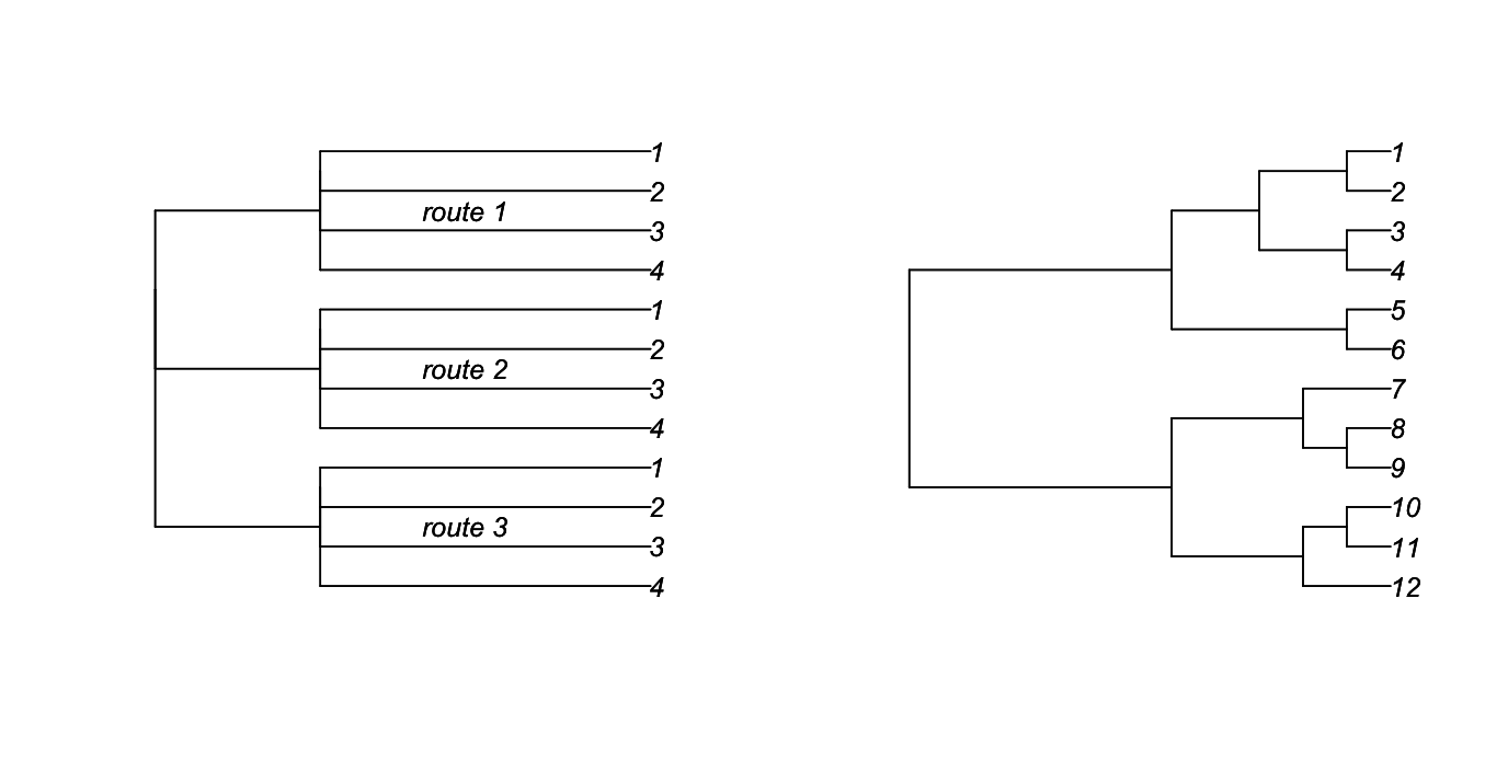
rtree() function in ape.A phylogeny can be graphed in a similar way, with the covariance between the species at the tips of the phylogeny equal to the height of the node of their most recent common ancestor. The phylogeny in the right panel of figure 3.1 corresponds to the covariance matrix
The comparison between the two phylogenies and their covariance matrices illustrates the similarity between hierarchical and phylogenetic data. They both have structured covariance matrices. In the case of hierarchical models, the matrices are often block diagonal, as they correspond to nested structures in the data. This is not necessary, however, and the logit normal-binomial model from Chapter 1 (subsection 1.4.4) is an example of a mixed model that does not have a block-diagonal covariance matrix. For phylogenetic models, the structure of the phylogeny forces the covariance matrix to be clustered, so that, for example, the covariance between species 1 and 3 is equal to the covariance between species 1 and 4, since species 1 had the same shared ancestor with species 3 and 4 (Fig. 3.1). I’ve shown an ultrametric phylogenetic, in which all tips are contemporaneous. It is also possible to have all tips ending at different distances from the base of the tree; in fact, this is the most common situation for phylogenies derived from molecular genetic data.
3.3.2 The strength of phylogenetic signal
Because the strength of phylogenetic signal – the magnitude of correlations among related species – varies among traits and groups of species, a statistical model needs to allow the strength of phylogenetic signal to vary. For the simple hierarchical data in figure 3.1 (left panel), the magnitude of correlations depends on the magnitude of the random effect variance relative to the residual variance; the larger the random-effect variance, the greater the hierarchical correlation. To allow a similar gradation for the strength of phylogenetic signal, branch-length transforms are used to push the locations of the internal nodes of the phylogeny either towards the tips (increasing phylogenetic signal) or towards the base (decreasing phylogenetic signal). The two most common branch-length transforms are Pagel’s λ (Pagel 1997, 1999) and the Ornstein Uhlenbeck (OU) transform (Martins and Hansen 1997).
Pagel’s λ transform involves reducing the height of the phylogeny by a factor λ and adding length to the tip branches by a factor (1 - λ), as shown in figure 3.2. This branch-length transform is similar to the structure of mixed models in which the random effect variance is reduced relative to the error variance, which extends the relative length of the tip branches.
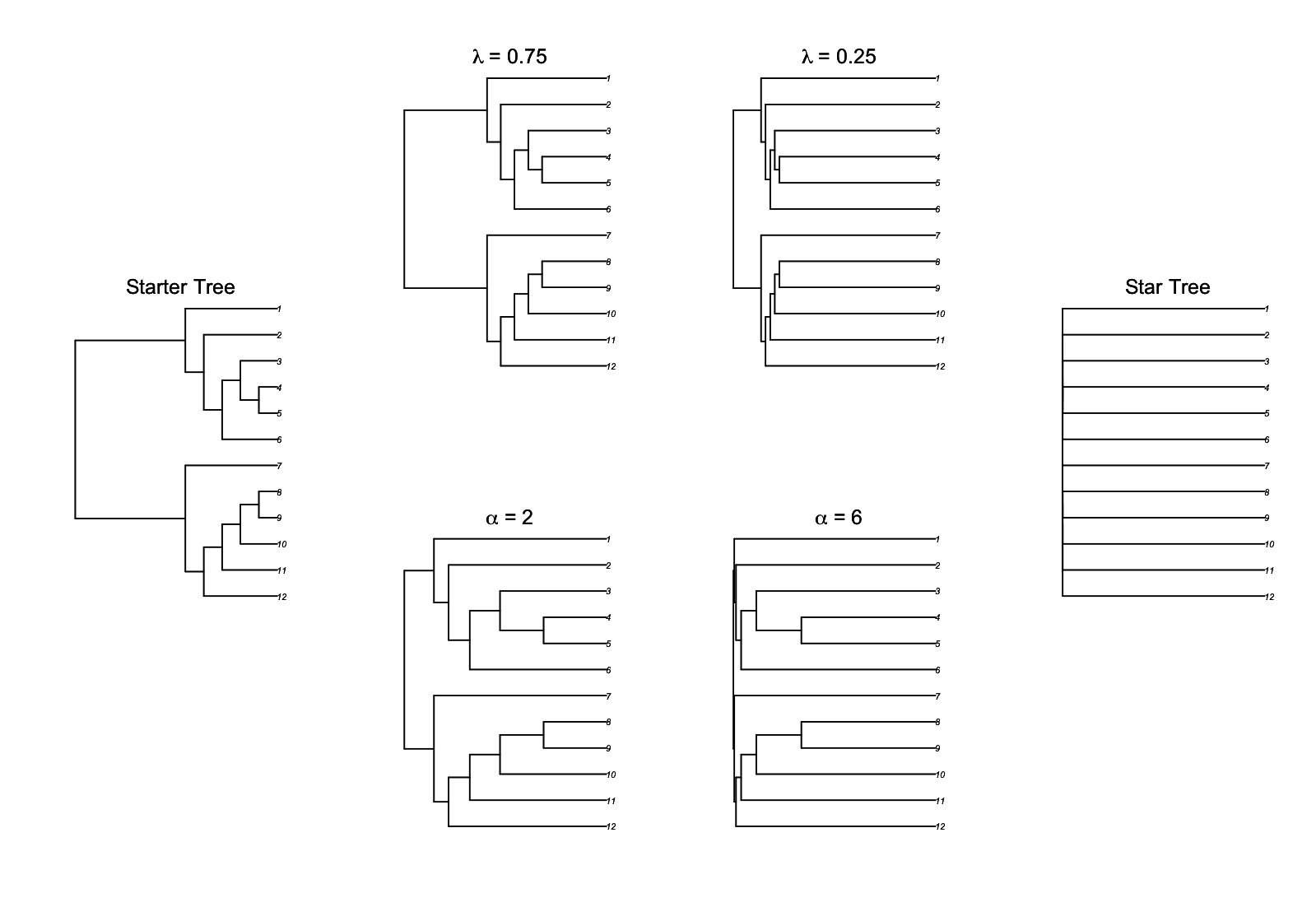
The second common branch-length transform, the OU transform, has different variants in the literature. The one I prefer is derived so that when its parameter d is zero (no signal) a “star” phylogeny is given in which all branches radiate from the base and there is no correlation between tips; when d is one, the original “starter” phylogeny is given. This formulation of the OU transform was what we used in Blomberg et al. (2003). However, the more common version in R packages has a parameter α that is inversely related to the strength of phylogenetic signal; when α = 0, there is strong phylogenetic signal, while as α increases to infinity a star phylogeny is given in which there is no covariance among species. As another complication, the original OU transform in Martins and Hansen (1997) and implemented in the package ape assumes that the trait value at the root of the phylogeny is not fixed, so that there are no zero elements in the covariance matrix, and the original starter tree is not recovered when α = 0. Here I use the OU transform implemented in phylolm() that does recover the starter phylogeny when α = 0. Figure 3.2 shows this transform paralleling Pagel’s λ transform; although they both change the strength of phylogenetic signal, they do this somewhat differently, with the OU transform tending to shorten branch lengths towards the base of the phylogeny more than Pagel’s λ transform.
3.3.3 Brownian motion evolution
Translating a phylogeny into a covariance matrix is generally described in the literature in terms of a “model of evolution”, so I will break my silence on evolution briefly in this subsection. Earlier I asserted that a phylogeny was a visual depiction of a covariance matrix. It is, but there is more to this association than visual. Phylogenies, as depicted by trees, give information about genetic diversification if they are generated from molecular data; morphological diversification if they are generated from trait data; or time if they are calibrated with the fossil record. There is a mathematical way to take a phylogeny and generate a covariance matrix. Specifically, if a hypothetical trait evolves in a Brownian motion fashion, increasing or decreasing a very small amount every very small time step up the phylogenetic tree, then the trait value will follow a stochastic random walk that branches at each node on the tree. Such as random walk has the property that the variance increases linearly with time. This means that the branch lengths on the phylogenetic tree are proportional to the variances and covariances of trait values among species. Thus, “Brownian motion evolution” gives a direct translation from phylogeny to covariance matrix.
The OU branch-length transform also is derived from a model of evolution. In the OU case, the model involves stabilizing selection to a global optimum. This stabilizing selection tends to erase the history of trait values; as time progresses, the stabilization exerts more influence as it bounds trait values around the optimum, so the values “forget” their starting points. Stated another way, the variance in trait values decelerates through time, so covariances in the distant past are reduced. This decrease of phylogenetic covariances can be modeled on the starter tree as OU evolution, or the starter tree can have its branch lengths transformed according to an OU process and then the phylogenetic covariances modeled as a Brownian motion process. Throughout this chapter, for clarity I’ll use the latter approach of first performing a branch-length transform and then pulling variances and covariances from the resulting covariance matrix under the assumption of a Brownian motion process.
3.4 Estimating phylogenetic signal
Phylogenetic signal can be estimated from a dataset and accompanying phylogeny as the value of the branch-length transform parameter (e.g., λ or α). This can be done with or without predictor variables in the model. I’ll first present the general regression model and then discuss the estimation of phylogenetic signal parameters, first for the case in which there are no predictor variables. When there are no predictor variables, the model gives a direct estimate of phylogenetic signal.
3.4.1 Phylogenetic regression model
A phylogenetic regression model for a single predictor variable is
Y = b0 + b1*x + e
e ~ norm(0, s2*V(θ))
Here, the covariance matrix of the errors, V(θ), contains the phylogenetic covariances and a phylogenetic signal parameter θ that could be λ or α. In contrast to a mixed model which would have two covariance matrices, one for the random effect and a second for the errors, the phylogenetic regression model might only have a single covariance matrix. However, for Pagel’s λ transform, the covariance matrix V(λ) can be written as the sum of two matrices, λ*V + (1 - λ)*I where V is the starter covariance matrix (typically the one derived assuming Brownian motion evolution) and I is the identity matrix.
This phylogenetic regression model is often referred to as a Phylogenetic Generalized Least-Squares model (PGLS). Technically, because the covariance matrix contains a parameter θ that must be estimated, this is really an Estimated GLS model (EGLS). Because a well-used package for fitting EGLSs is nlme, in which the function gls() solves the EGLS problem, I’m not going to fight the usage of PGLS. The important point, though, is that simple GLS can’t be used for estimating parameter values. Instead, ML or REML are generally used, although there are alternatives (Ives et al. 2007). For this specific model, ML or REML will give estimates of the regression coefficients (b0 and b1), the phylogenetic signal (θ), and s2 that scales the residual variance.
Of course, this regression model can be expanded to include multiple predictor variables, and interactions among them. Unlike hierarchical models, however, there is typically only a single parameter that is estimated in the covariance matrix. Exceptions to this are models that attempt to identify regions of the phylogeny in which changes in trait evolution are relatively fast or slow, or where there has been a shift in the optimum trait value governing an OU process (Butler and King 2004, Bartoszek et al. 2012). I won’t talk about these models in this book, because they involve both statistical and conceptual challenges; I would only attempt this type of analyses with very large numbers (many hundreds) of species and a very clear a priori hypothesis for how the rate of trait evolution might vary.
For the case without a predictor variable x, figure 3.3 gives a simulated example, with branches colored according to a hypothetical trait evolving in a Brownian motion fashion up a phylogeny. The tip trait values are plotted in the panel on the right. The clustering of points reflecting phylogenetic correlations is clear.
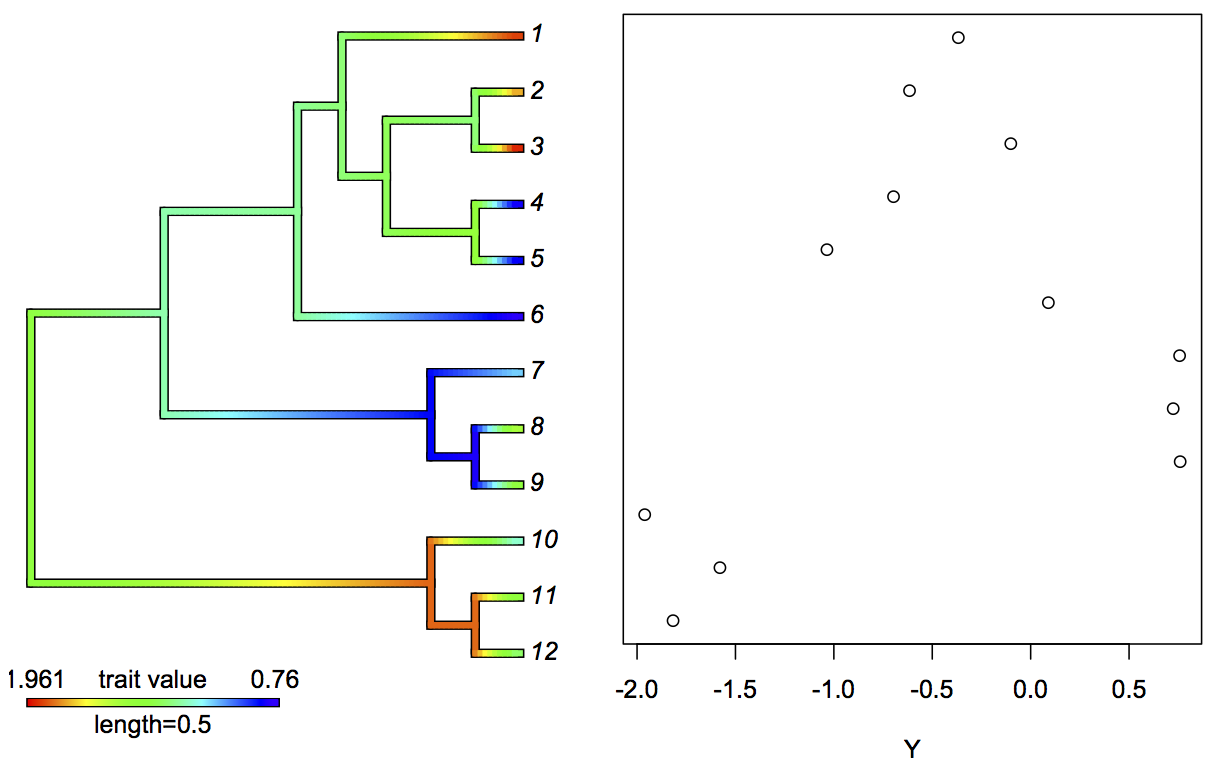
phytools package (Revell 2012). The right panel gives the trait values at the tips of the phylogeny.3.4.2 Analyzing hierarchical data as a phylogeny
To hammer home the close relationship between hierarchical and phylogenetic models, I fit simulated hierarchical data using both a LMM and a phylogenetic model. The hierarchical data and LMM have the same structure as the hierarchical data in figure 3.1, with stations nested within routes. The phylogenetic model requires constructing a “phylogeny” for the hierarchical data, which involves taking the covariance matrix suitable for stations nested within routes and converting it into a phylogenetic object of class phylo in the package ape (Paradis et al. 2004). For this illustration, I simulated data for 4 routes each containing 6 stations (Fig. 3.4).
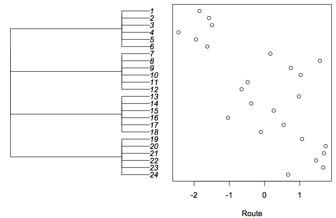
I fit the phylogenetic model using Pagel’s λ branch-length transformation, since this takes the form of the sum of a phylogenetic covariance matrix and the identity matrix, which has the same form as the covariance matrix for the LMM with a random effect for route (although parameterized differently, since the phylogenetic covariance matrices are multiplied by λ and (1-λ), while the LMM matrices are multiplied by 1 and s2_b). The results from the LMM and PGLS are
# Fit using lmer()
z.lmm <- lmer(Y ~ 1 + (1|route), REML=F, data=d)
summary(z.lmm)

     AIC      BIC   logLik deviance df.resid
    63.8     67.4    -28.9     57.8       21

Random effects:
 Groups   Name        Variance Std.Dev.
 route    (Intercept) 1.2823   1.1324
 Residual             0.3935   0.6273
Number of obs: 24, groups:  route, 4

# Fit using phylolm()
z.pgls <- phylolm(Y ~ 1, phy=phy.lm, model = "lambda", data=d)
summary(z.pgls)

   AIC logLik
 63.82 -28.91

Parameter estimate(s) using ML:
lambda : 0.9564764
sigma2: 1.675826

# For the PGLS, the route-level variance is lambda*vcv[2,1]*sigma2
cov.pgls <- z.pgls$optpar * vcv[2,1] * z.pgls$sigma2
cov.lmm <- summary(z.lmm)$varcor[[1]][1]
c(cov.pgls, cov.lmm)
[1] 1.28231  1.28231
The logLik of both models is the same, indicating that they fit the data the same. Showing that the covariance for stations within routes are the same involves extracting the covariance from the phylogenetic covariance matrix, vcv. This is given by λ (= z.pgls$optpar) times the covariance in vcv (I just picked the element in the second row, first column, vcv[2,1]) and the estimate of the overall variance s2 (= z.pgls$sigma2). That the covariances for stations within routes are the same for the LMM and PGLS demonstrates that they are the same model.
3.4.3 Choosing a branch-length transform
Given the several possible branch-length transforms that could be used to assess phylogenetic signal, how do you select the best? An appropriate way is to use the likelihood of the fitted model. As discussed in subsection 2.3.2, the likelihood gives the probability of observing the data conditional on the values used for the parameters in a model. When these parameters are fit by ML, the likelihood of the resulting model is the highest possible for the given branch-length transform. Therefore, if one branch-length transform allows the model to fit the data better than another branch-length transform, then its likelihood will be higher.
To illustrate this, I first simulated a phylogeny using the rtree() function in ape, additionally using the function compute.brlen() with a Grafen branch-length transformation to make it ultrametric. I used the transf.branch.lengths() function from phylolm() (Ho and Ane 2014) to transform the branch lengths according to Pagel’s λ, and simulated data using rTraitCont() in ape. Finally, I fit the simulated data using phylolm() using either Pagel’s λ (model = "lambda") or the OU branch-length transform (model = "OUfixedRoot"). Below, I’ve abbreviated the output to show the important results.
<- 100
phy <- compute.brlen(rtree(n=n), method = "Grafen", power = 1)
# Simulate data with Pagel's lambda
lam <- .5
phy.lam <- transf.branch.lengths(phy=phy, model="lambda",
parameters=list(lambda = lam))$tree
Y <- rTraitCont(phy.lam, model = "BM", sigma = 1)
summary(phylolm(Y ~ 1, phy=phy, model = "lambda"))
AIC logLik
238.6 -116.3
lambda : 0.5563776
sigma2: 1.036665
summary(phylolm(Y ~ 1, phy=phy, model = "OUfixedRoot"))
AIC logLik
251.9 -122.9
alpha: 31.35936
sigma2: 48.83051
phylolm() gives the fitted measure of phylogenetic signal (lambda or alpha) that transforms the covariance matrix, and sigma2 that scales the covariance matrix. Because the branch-length transforms change the variances in the covariance matrices, the estimates of sigma2 can’t be compared. However, the log likelihood logLik is clearly higher for the model fit with Pagel’s λ, indicating that this is the better of the two branch-length transforms.
Repeating these simulations 100 times shows that the branch-length transform used to simulate the data isn’t always the one that gives the better fit to the simulated data. Even for n = 100 species, 7% of the datasets simulated with λ = 0.5 were fit better using an OU branch-length transform, and when the data were simulated with an OU branch-length transform with α = 1, 16% of the simulated datasets were fit better using Pagel’s λ. This is a indication that it is often difficult to fit details of the covariance matrix: covariances can be hard to estimate.
3.5. Statistical tests for phylogenetic signal
There are multiple ways of testing for the presence of phylogenetic signal in a dataset. Somewhat surprisingly, most ways that are available in common packages in R do not have great statistical properties: most have low statistical power. Here I present methods that I discussed in chapter 2: the Likelihood Ratio Test (LRT), a parametric bootstrap of the phylogenetic signal parameter, and a parametric bootstrap of the null hypothesis H0 that there is no phylogenetic signal. I’ll also introduce a permutation test and Blomberg’s K. For all of these examples, I’ll analyze the same dataset that I generated by simulation to have moderately strong phylogenetic signal (λ = 0.5) using the code
<- 30
phy <- compute.brlen(rtree(n=n), method = "Grafen", power = 1)
lam <- 0.5
phy.lam <- transf.branch.lengths(phy=phy, model="lambda",
parameters=list(lambda = lam))$tree
Y <- rTraitCont(phy.lam, model = "BM", sigma = 1)
3.5.1 Likelihood Ratio Test
I introduced the Likelihood Ratio Test (LRT) in subsection 2.6.2 as a general method to test the significance of a component of a model by comparing the full model containing that component to the reduced model without the component. In subsection 2.6.2, the parameter in question was a regression coefficient, but LRTs can also be used to give P-values in statistical tests of phylogenetic signal that involve the covariances of the errors. For this, the LRT compares a full model in which phylogenetic signal is estimated using ML to the reduced model in which there is no phylogenetic signal; the appropriate reduced model here is just a LM. Twice the log of the likelihood ratio (LLR) between models is asymptotically (as n gets large) chi-square distributed. The LRT is a standard way to generate P-values, although we’ll find below that they are prone to deflated type I errors and loss of power for small sample sizes. For the simulated dataset used in the following examples, LRTs for Pagel’s λ and the OU transforms were P = 0.12 and P = 0.22, respectively.
3.5.2 Parametric bootstrap of the parameter
It is possible to test for phylogenetic signal by performing a parametric bootstrap of the estimator of the phylogenetic signal parameter. This bootstrap gives the approximate distribution of the estimator from which P-values can be derived. The procedure of the parametric bootstrap is (subsection 2.6.3):
- Fit the model to the data.
- Using the estimated parameter value of interest, simulate a large number of datasets.
- Refit the model to each simulated dataset.
- The resulting distribution of the parameter values estimated from the simulated datasets approximates the distribution of the estimator, allowing P-values to be calculated.
phylolm() will perform this bootstrap for you automatically when you specify a number for boot.
The bootstrap of the parameter can lead to incorrect P-values when the estimator is biased (subsection 2.6.3). This turns out to be the case for the estimator of phylogenetic signal (Fig. 3.5). The estimates of λ and α are biased towards less phylogenetic signal (lower λ and higher α) than used to simulate the bootstrap datasets. This is seen in Fig. 3.5: the mean of the parameter estimates (λ and α) given by the green lines are closer to the value of no signal (λ = 0 and α = 50, the upper limit of α in phylolm) than the value used to simulate the data given by the red line. This underestimate of the phylogenetic signal is anticipated to lead to type I errors that are too low and a corresponding loss of statistical power to detect phylogenetic signal.
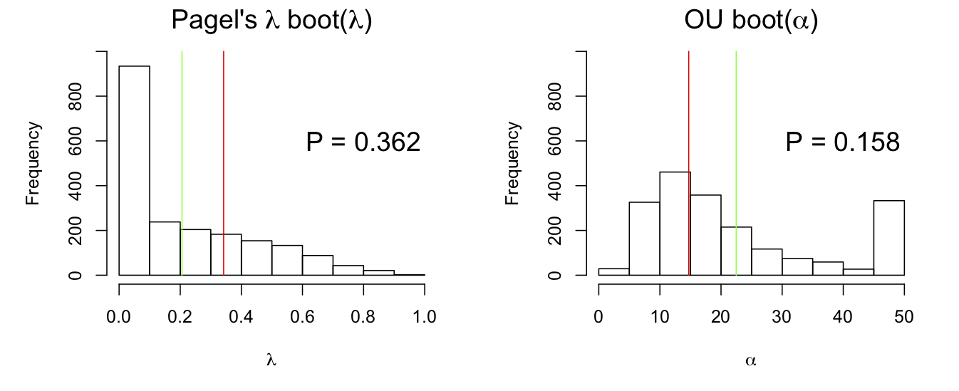
phylolm() for a simulated dataset. The red lines give the value of the phylogenetic signal parameter used to bootstrap the data, and the green lines are the means of the estimates.Note that the bootstrap estimates of λ and α tend to cluster at values giving no signal (λ = 0 and α = 50). This is typical for estimates of phylogenetic signal, and in general for ML estimates of variance components of models for correlated data. For ML estimation of variances and covariances when they are weak, there is often a peak in the likelihood function at zero, leading to estimates of zero. This type of absorption at zero (no phylogenetic signal) underlies the bias in the estimates of phylogenetic signal found for the parametric bootstrap of the estimator (Fig. 3.5).
3.5.3 Parametric bootstrap of H0
The parametric bootstrap of H0 involves the following procedure (subsection 2.6.4):
- Fit the model to the data and calculate the log likelihood ratio (LLR) between the full model and the reduced model without the parameter of interest.
- Using the estimated parameters from the reduced model, simulate a large number of datasets.
- Refit both the full and reduced models for each dataset and calculate the LLR.
- The resulting distribution of LLRs estimated from the simulated datasets approximates the distribution of the estimator of the LLR, allowing P-values to be calculated.
This bootstrap is related to a LRT, but rather than approximate the distribution of 2*LLR by a chi-square distribution, the distribution is obtained by parametric bootstrapping.
Figure 3.6 shows the bootstrap estimates of 2*LLR for simulations under H0. Under the standard LRT, these distributions should be chi-square (blue lines), which they are not. This is due to the absorption of estimates for no phylogenetic signal, which is observed in the mass of values of LLR close to zero. This does not necessarily mean that the parametric bootstrap of H0 is wrong; this absorption at zero occurs under the null hypothesis that there is no phylogenetic signal. Instead, the comparison between the parametric bootstrap of H0 shows that the chi-square approximation is poor, because it fails to account for the tendency of the estimator to absorb at zero.
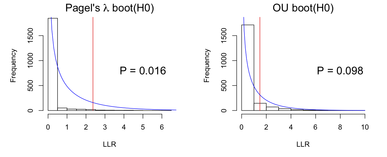
*LLR for Pagel’s λ and OU models under the null hypothesis that there is no phylogenetic signal. Simulated data were fit using phylolm(). A chi-square distribution with df = 1 is shown by the blue line.3.5.4 Permutation test
A permutation test can be performed that is very similar to the parametric bootstrap of H0. In general, permutation tests are the gold standard for testing null hypotheses involving correlations among data. In this case, under the null hypothesis that there is no phylogenetic correlation, trait values can be randomly permuted among species without changing the structure of the data. Thus, the permutation test involves generating a large number of permutation datasets, fitting each with a model for phylogenetic signal, and calculating P-values from the fraction of estimates that are more extreme than the estimate from the original dataset. Using a permutation test for the data we’ve been analyzing (Fig. 3.7) gives distributions of estimates of λ and α very similar to those obtained with the parametric bootstrap of H0 (Fig. 3.6), and very similar P-values.
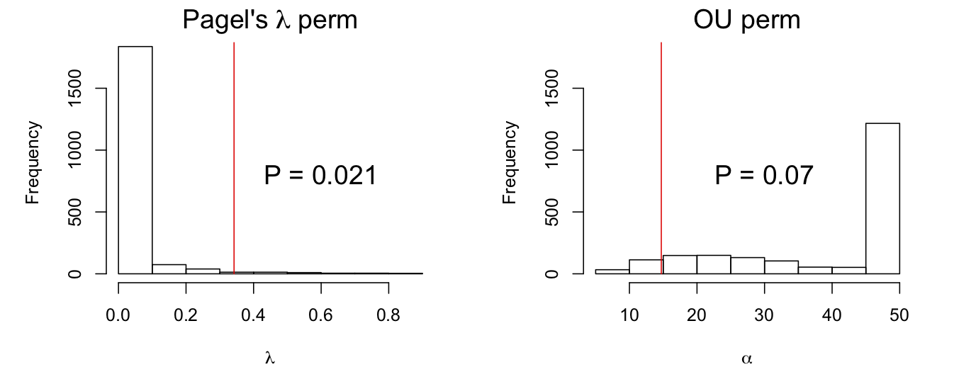
phylolm() by permuting values of Y among species under the null hypotheses that there is no phylogenetic signal. The red lines give the “true” value of the phylogenetic signal parameters estimated from the data.I need to give a short digression about the conceptual differences between bootstraps and permutation tests. First, the bootstrap tests I’ve been using so far have all been parametric bootstraps, in which a model is fit and datasets simulated from the fitted model. “Parametric” refers to the fact that a specific distribution has to be used to simulate the errors. The standard bootstrap is the non-parametric bootstrap (or simply “bootstrap” without the “non-parametric”). In the non-parametric bootstrap, there is no assumption about the distribution of errors. Instead, the actual residuals from the fitted model are used as the errors to generate the bootstrap datasets. For the tests of phylogenetic signal, this would involve fitting the model (the very simple model with only an intercept), collecting the residuals (differences from the mean), and for each species selecting from these residuals with replacement to construct the bootstrap datasets. The only difference between this procedure and the permutation is that the bootstrap resamples the residuals with replacement, whereas the permutation resamples residuals without replacement (since permuting residuals around the mean is the same as permuting the values).
Although the only difference between non-parametric bootstrap tests and permutation tests is that the former resamples with replacement and the latter resamples without replacement, the interpretation of these tests is different (Efron and Tibshirani 1993). The non-parametric bootstrap, as with the parametric bootstrap, gives an approximation of the distribution of the statistical estimator for the parameter in question under H0. The heuristic justification for this is that the residuals from a fitted model give n realizations of the true process underlying the experiment, and therefore they can be resampled as if they were the complete distribution in order to derive the distribution of the estimator. The permutation test does not involve any thought of the estimator or statistical inference about the process underlying the data. Instead, the permutation test asks what the probability is of observing the pattern in the data under the assumption it is random (as given by the permutation). In short, bootstrapping gives an approximation of the estimator while a permutation test gives a probability of an outcome.
I have focused on bootstraps in this book rather than permutation tests, because a major goal is to explain statistical inference, which involves understanding the processes that generate data. Bootstraps directly involve inference about statistical processes. Furthermore, I’ve used parametric bootstraps rather than non-parametric bootstraps. A non-parametric bootstrap could easily have been performed for testing for phylogenetic signal. A limitation of non-parametric bootstrapping often arises in hierarchical data, however, because it is impossible to derive a non-parametric resampling scheme for the residuals to test a null hypothesis of interest. For example, suppose you wanted to test the significance of a regression coefficient in a GLMM, such as testing for the effect of the variable WIND on station-level observations of grouse (subsection 1.5.4). Because the residual errors are not independent (observations from stations within the same route are correlated), the residuals can’t be resampled independently to construct the bootstrap datasets. An added problem in this example is that the observations are binary (grouse present or absent), so the residuals can’t be resampled in a way to retain binary values of the observations. Thus, parametric bootstrapping is possible even when non-parametric bootstrapping is impossible, either due to correlations in the residual errors that need to be preserved for the statistical test, or due to the discreteness of the data.
3.5.5 Blomberg’s K
Blomberg’s K is a metric of phylogenetic signal. This is distinct from a model, such as a PGLS with a Pagel’s λ or an OU branch-length transform that gives a parameter (λ or α) corresponding to phylogenetic signal. The PGLS requires a model based on a stochastic process that is thought to underlie the data; the model provides enough information to simulate the data. In contrast, metrics are values computed from the data without making assumptions about the underlying stochastic process generating the data. Calculating a metric like Blomberg’s K does not lead to a model that can be used to simulate the data.
We designed Blomberg’s K around the mean-squared-error (MSE) of the data (Blomberg et al. 2003). If there is no phylogenetic correlation among the residuals R, then the variance of the residuals is measured by the OLS MSE, which is computed by taking the sum of the squared residuals and dividing by (n - 1). If there is phylogenetic signal, then the variance of the residuals is measured by the Generalized Least squares (GLS) MSE that depends on the covariance matrix V derived from the phylogeny:
MSE = (1/(n - 1))*(R’ %*% iV %*% R)
where R is the n x 1 vector of residuals, R’ is the transpose of R, iV is the inverse of the matrix V, and %*% is matrix multiplication. Thus, the squared residuals are weighted by the elements of iV to account for the correlation in the data. (A more-detailed explanation is presented in Blomberg et al. 2003.) To distinguish two MSEs, let MSE(star) be the OLS MSE that assumes no phylogenetic signal (the phylogeny is a “star” with equal branch lengths radiating from the base), and let MSE(phy) be the GLS MSE calculated using the phylogeny to compute V.
Blomberg’s K is based on the ratio MSE(star)/MSE(phy). If there is correlation in the residual errors, then MSE(star) decreases relative to MSE(phy), decreasing the ratio MSE(star)/MSE(phy). The ratio also depends on the number of species and the topology of the phylogeny. Therefore, we standardized MSE(star)/MSE(phy) by its expected value if the phylogenetic correlations were in fact given by V. Thus, if phylogenetic signal is the same as the phylogenetic covariance matrix V, then K = 1. Values smaller than 1 imply weaker phylogenetic signal, and values greater than 1 imply stronger phylogenetic signal. The only value of K that has a clear interpretation is K = 1. Even with the standardization relative to the expectation if the residuals had covariance matrix V, the value of K when K ≠ 1 still depends on the specific phylogenetic tree; therefore, it is not particularly useful to compare values of K among datasets from different phylogenies. Nonetheless, Blomberg’s K is useful as a metric that doesn’t make parametric assumptions about the distribution of the residual errors: the MSEs used in K are from OLS and GLS which do not assume that the errors are normally distributed. While it is true that, if traits evolved by Brownian motion up a phylogenetic tree, then the distribution of traits at the tips would be a multivariate normal distribution with covariance matrix V, this is not a prerequisite for K to measure phylogenetic signal.
The null hypothesis that there is no phylogenetic signal can be tested using Blomberg’s K in a permutation test. Trait values are permuted among tips, and the resulting distribution of K is compared to the value of K calculated from the data. This permutation test is performed by the function phylosig() in the package phytools, and for the dataset we are analyzing, P = 0.018. Even though this is the same permutation test used to test for phylogenetic signal with Pagel’s λ and the OU branch-length transforms (subsection 3.5.4), the results need not be the same. Blomberg’s K uses different characteristics of the data than Pagel’s λ and OU transforms, just as Pagel’s λ and OU themselves make different assumptions about the exact form of the covariances (subsection 3.4.3). Therefore, all three might give somewhat different P-values.
3.5.6 Type I errors and power for tests of phylogenetic signal
To assess type I errors and statistical power of different methods for identifying phylogenetic signal, I simulated data with increasing phylogenetic signal using either Pagel’s λ or OU branch-length transform (Fig. 3.8). I then tested for phylogenetic signal using Pagel’s λ and OU transforms with a LRT, Pagel’s λ and OU transforms using a bootstrap test of H0, and Blomberg’s K using a permutation test. I didn’t test for phylogenetic signal using the bootstrap of parameter estimates, because we know from subsection 3.5.2 that the estimates of λ and α are biased towards low estimates of phylogenetic signal, and therefore they will likely have low power. In these simulations, I used the same starter phylogeny because this made it possible to calculate a single bootstrap approximation of the distribution of the estimators of λ and α under H0. If instead a different phylogeny was used for each simulation, then a separate bootstrap distribution of LLR would have to be computed for each simulated dataset, because the null distributions of LLR for the Pagel’s λ and OU models could depend on the phylogeny. The overall conclusions, however, are likely to be the same if I had used a randomly constructed phylogeny for each simulated dataset.
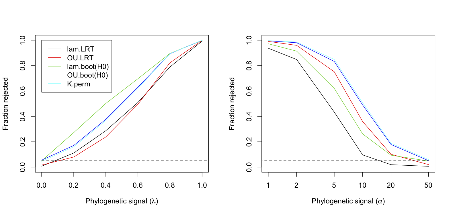
Several conclusions are apparent in figure 3.8. First, when data are simulated using Pagel’s λ branch-length transform (left panel), then the bootstrap LRT using this transform has the greatest power. Similarly, when data are simulated with an OU branch-length transform (right panel), then the bootstrap LRT using this transform has greater power than the bootstrap LRT using Pagel’s λ. This shows that the two branch-length transforms are generating different covariance patterns in the data, and the statistical test that matches the actual covariance pattern has the greater power. Second, the results for the permutation test with Blomberg’s K are almost identical to the results for the bootstrap test using the OU transform. Therefore, Blomberg’s K and the OU transform are picking up similar patterns in the phylogenetic covariances. Third, the standard LRTs that use a chi-square to approximate the distribution of LLRs generally had low power. The only case in which the standard LRT outperformed a bootstrap LRT was when data were simulated with the OU transform; in this case, the standard LRT using the OU transform outperformed the bootstrap LRT using Pagel’s λ transform (right panel).
These patterns of statistical power underscore that “phylogenetic signal” is not a single, simple quantity. Phylogenetic signal refers to covariances in trait values among species, but the relative magnitude of these covariances can take different forms. Different methods will differ in their power to detect these different forms of phylogenetic signal.
3.6 Estimating regression coefficients
The preceding analyses target phylogenetic signal which is part of the variance component of the phylogenetic models. The regression coefficients are part of the mean component of the models. To investigate estimation of regression coefficients in phylogenetic models, I simulated data using the regression model introduced in subsection 3.4.1. This regression model with one predictor variable can be simulated and fit as follows:
<- 20
b0 <- 0
b1 <- .5
lam.x <- 1
lam.e <- .5
phy <- compute.brlen(rtree(n=n), method = "Grafen", power = 1)
phy.x <- transf.branch.lengths(phy=phy, model="lambda",
parameters=list(lambda = lam.x))$tree
phy.e <- transf.branch.lengths(phy=phy, model="lambda",
parameters=list(lambda = lam.e))$tree
x <- rTraitCont(phy.x, model = "BM", sigma = 1)
e <- rTraitCont(phy.e, model = "BM", sigma = 1)
x <- x[match(names(e), names(x))]
Y <- b0 + b1 * x + e
Y <- array(Y)
rownames(Y) <- phy$tip.label
# Fit with phylogenetic correlations
summary(phylolm(Y ~ x, phy=phy, model = "lambda"))
# Fit without phylogenetic correlations
summary(lm(Y ~ x))
Here, separate phylogenies allow different strengths of phylogenetic signal for the predictor variables x and the residual error e. Specifically, phy.x and phy.e are derived using transf.branch.lengths(). rTraitCont() is used to simulate both x and e, which lead to simulated values of Y. The line x <- x[match(names(e), names(x))] is used to make sure the species order in x is the same as the order in e, with the function match() aligning the index of x so that the names of e and x are in the same order. Y needs to be an array, and it has to have rownames giving the species names in the phylogeny. In general for phylogenetic analyses in R, you have to be careful to make sure that the data points match the species they correspond to. Different functions handle this differently, but phylolm() will tell you if it hasn’t found rownames in the data.frame to match the species names in the tip.label vector of the phylogeny.
The simulated data are fit both to a phylogenetic model using Pagel’s λ transformation, and to a LM that does not account for phylogenetic signal. I suggest you spend a little time running the simulations and fitting the data to see how different strengths of phylogenetic signal in x and e (lam.x and lam.e) affect the results.
3.6.1 Where phylogenetic signal comes from
The models that we were using to estimate phylogenetic signal in Y (section 3.5) were regression models with only an intercept. In these models, the source of phylogenetic signal in the residual errors was the phylogenetic relatedness of species. For the phylogenetic regression with predictor variables, the source of phylogenetic signal in the residual errors is not as obvious. This phylogenetic signal is in the variance in Y that is not explained by the predictor variable x. There are ways in which phylogenetic signal can be generated in a process involving only Y and x: if evolution of x through time represents a moving optimum for the evolution of Y, then an evolutionary lag of Y behind x can generate a phylogenetic signal in the residual error (Hansen and Orzack 2005). To me this seems like a pretty specialized situation that is unlikely to explain the ubiquity of phylogenetic signal in regression models; phylogenetic signal in the residual variation in regression models is found across a wide range of data. A simpler and (I guess) more likely explanation is that the regression model excludes other predictor variables that themselves show phylogenetic signal. Since they are not included in the model, their effects appear in the residual variation as phylogenetic signal. Thus, the regression model could be written
Y = b0 + b1*x + u1 + u2 + e
u1 ~ norm(0, s2_u1*V(θ_u1))
u2 ~ norm(0, s2_u2*V(θ_u2))
e ~ norm(0, s2_e*I)
Here, there is residual variation in e that has no phylogenetic signal, and two unmeasured traits u1 and u2 that have phylogenetic signal. Since they are not measured, the apparent residual variation is u1 + u2 + e, which has phylogenetic signal. Of course, there might be only one unmeasured trait u1, or there might be many more than two.
You might think that if there are many unmeasured traits, then their phylogenetic signals will cancel each other out: for example, two related species might have high values of u1 and low values of u2, which would degrade the overall phylogenetic signal from u1 + u2. This turns out not to be the case. If u1 and u2 are independent of each other, then the variance in u1 + u2 for species i is
var[u1(i) + u2(i)]
= var[u1(i)] + var[u2(i)].
The covariance in u1 + u2 between species i and j is
cov[u1(i) + u2(i), u1(j) + u2(j)]
= cov[u1(i), u1(j)] + cov[u2(i), u2(j)].
Therefore, if u1 and u2 have the same covariance matrix, the covariance matrix for u1 + u2 is just two times the covariance matrix for either one of them. This means that having multiple unmeasured traits doesn’t degrade the phylogenetic signal in the unexplained variation. The algebra gets a little more involved if u1 and u2 have different covariance matrices, or if u1 and u2 are themselves correlated, but these cases don’t overturn the conclusion that phylogenetic signal isn’t lost – it is just a weighted average (weighted by the variance scalars s2_u1 and s2_u2) of the phylogenetic signals of u1 and u2.
3.6.2 Type I errors and power
Not surprisingly, type I errors and power in detecting statistically significant regression coefficients are affected by phylogenetic correlations in the errors. What is maybe more surprising is that type I error and power are strongly affected by phylogenetic signal in x; this is shown nicely by Revell (2010). The reason this might be surprising is that, in standard regression, the distribution of the predictor variables is not important: in OLS, there is no assumption about how the predictor variables are distributed, and other than making sure there are no outlying points with high leverage, the distribution of x can be ignored. For phylogenetic regression, however, the distribution of x comes into play in two ways. First, it can affect the statistical power to detect significant effects of a predictor variable. This is not a problem per se, since it is just an indication that the predictor variable contains less information if it has phylogenetic signal. Second, phylogenetic signal in a predictor variable magnifies the problems of mis-specifying the phylogenetic signal in the errors, leading to inflated type I errors. This is strictly speaking not a problem, since you should hope that you have correctly specified the phylogenetic signal of the errors. But this is a potential problem to be aware of.
To illustrate these two effects of phylogenetic signal in x, I simulated datasets for different values of b1 without and with phylogenetic signal in x. I then tested the rejection rates of the null hypothesis H0:b1 = 0 for a PGLS using a Wald test, a LM using a t-test, and a PGLS using a bootstrapped LRT under the null hypothesis. For the case of no phylogenetic signal in x, all three methods had good type I error control. However, the LM had much lower power. For the case of phylogenetic signal in x, however, the LM had horrible type I error control. Even the PGLS using a Wald test had inflated type I errors, with the rejection rate of 0.064 when b1 = 0. Of course, the bootstrap LRT under H0 corrected this.
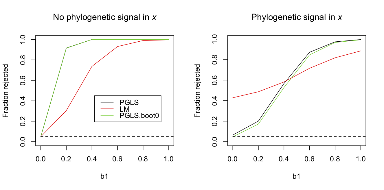
b0 = 0, s2.e = 1 and s2.x = 1It is disturbing that the PGLS didn’t have perfect type I error control. This is a pretty standard analysis in the evolutionary and statistical literatures. The simulations were performed all with the same phylogeny, since this makes it possible to use the same bootstrap thresholds on the likelihood ratio (otherwise, the bootstrap would be too computationally demanding). Therefore, this could be a problem that is worse for this particular phylogeny than you might expect for other phylogenies. However, using 10,000 simulations with random phylogenies selected for each, the rejection rate was 0.068, indicating that the inflated type I error rates are systemic. The best way to address this is to perform the bootstrap LRT under H0. Given that this is a routine analysis and I doubt many practitioners will use the bootstrap (even though they should), at least be skeptical of reported P-values for small sample sizes (although here “small” is n = 30).
3.6.3 Partial R2s
A final lesson from figure 3.9 is that phylogenetic signal in x decreases the power to test the null hypothesis that b1 equals zero; this is seen in comparing the results for the bootstrap PGLS between left and right panels. Explaining the cause of this decrease in power is a reason to introduce partial R2s applied to phylogenetic data.
A partial R2 measures how much explanatory power is lost when a component of a model is removed. The total R2 is the partial R2 when everything in a model is removed except for the intercept (mean). In OLS, the explanatory power of a model is measured by the proportion of the variance in Y that is explained by the model; it is just 1 - var[residuals]/var[Y]. For models with correlated data, there is no simple way of defining the proportion of the variance in Y explained by a model. Nonetheless, there are reasonable ways of defining R2 for mixed and phylogenetic models; I describe three in Ives (in press). Here, I will discuss the one that is based on the likelihoods, specifically
<- 1 - exp(-2*(logLik(mod.f) - logLik(mod.r))/n)
where mod.f is the full model and mod.r is the reduced model with the component of interest removed. Thus, for the partial R2 for x depends on the difference between the full model mod.f and the reduced model mod.x:
<- phylolm(y ~ x, phy=phy, model = "lambda")
mod.x <- phylolm(y ~ 1, phy=phy, model = "lambda")
I’ve used the notation of mod.x to denote the model without x, since this is the reduce model used to test the significance of x. The R2 for the phylogenetic signal in residuals can be computed from
<- phylolm(y ~ x, phy=phy, model = "lambda")
mod.phy <- lm(y ~ x)
To illustrate the partial R2s, I simulated two datasets similar to those in figure 3.9 with b0 = 0, b1 = 0.5, and phylogenetic signal in e given by lam.e = 0.8. Also, I increased n to 100 to reduce the variation from one simulation to the next and make the following table more representative of all simulations. The partial R2s for datasets simulated with and without phylogenetic signal in x were
| No signal in x | Signal in x | |||
| full model | reduced model | partial R2 | partial R2 | |
| 1 | Y ~ 1 + e(phy) | Y ~ 1 + e | 0.28 | 0.52 |
| 2 | Y ~ x + e(phy) | Y ~ 1 + e(phy) | 0.49 | 0.10 |
| 3 | Y ~ x + e(phy) | Y ~ 1 + e | 0.63 | 0.56 |
| 4 | Y ~ x + e(phy) | Y ~ x + e | 0.53 | 0.49 |
| 5 | Y ~ x + e | Y ~ 1 + e | 0.21 | 0.14 |
When there is no phylogenetic signal in x, the partial R2s for x (row 2) and the phylogenetic signal in e (row 4) are similar in magnitude. Furthermore, the total R2 for the model without x (row 1) and for the model without phylogenetic signal in e (row 5) are of similar magnitude. When there is phylogenetic signal in x, however, the partial R2 for x (row 2) is very low. This indicates that the inclusion of x in the model adds little explanatory power, as measured by the increases in the log likelihood. The partial R2 for phylogenetic signal in e (row 4), however, remains high. The reason for this is that, if x is removed from the model, the phylogenetic effect that x imparts on the residual variation is absorbed by the phylogenetic signal in e. This is possible, because the effects of x on Y will have phylogenetic signal that matches the phylogenetic signal in e. Note that the converse doesn’t happen: the partial R2 for phylogenetic signal in e doesn’t change much with phylogenetic signal in x. This is because the information lost by removing phylogenetic signal in e can’t be replaced by the phylogenetic signal in x; the patterns produced by x not only make phylogenetically related species have similar results, they also force them to be relatively large or small, depending on the values of x and b1. Therefore, even though residuals for related species might be correlated, phylogenetic signal in x can’t absorb this signal if values of x and b1 predict residuals in the opposite direction.
I didn’t see much value in deriving R2s for models for correlated data until I realized how partial R2s can be used to tease apart different components of a model to understand how predictor variables (fixed effects) interact with phylogenetic signal (random effects). Total R2s can be useful for comparing very different models fit to the same data, or in broad comparisons among many datasets. Nonetheless, total R2s don’t seem particularly useful as measures of goodness-of-fit of a model. In other words, I don’t think it is particularly useful to report R2s routinely for analyses with correlated data, even though many practitioners will likely feel this urge.
3.7 How good must the phylogeny be?
All of the phylogenetic analyses so far have assumed that the phylogeny is known without error. This conflicts with the common convention of publishing phylogenies with the associated uncertainty in their topologies: typically the bootstrap confidence in the topology at each node is reported, measured by the frequency in a bootstrap analysis of the phylogeny construction that the best-supported node appears in the bootstrapped phylogenies. I don’t know of a detailed, systematic simulation analysis of how uncertainty in phylogenetic tree topology and branch lengths affect inference using models for comparative data, but Martins (1996) and Rangel et al. (2015) outline general approaches for this problem very nicely. In this section, I thought I’d present a simulation that introduces this as a potential problem for your analyses.
The simulations are based on a simple phylogenetic regression model with a single predictor variable x and phylogenetic signal in the residual errors. For each simulation, I generated a random phylogeny and simulated data either with or without phylogenetic signal in x. I fit the model using phylolm() with Pagel’s λ branch-length transformation and scored whether the null hypothesis H0:b1 = 0 was rejected using a Wald test. I then took the phylogeny and degraded it by permuting species among tips of the phylogenetic within clades of different depths. For example, if the clade contained only three species, then the permutation could result at most in the change of a single node (i.e., A and B might initially have been more closely related, while after permutation B and C are most closely related). The number of nodes that were changed by these permutations at different depths was scored by the Robinson and Foulds distance (Robinson and Foulds 1981), RF, divided by 2 (since the RF distance takes on values of even integers). I continued to permute species within clades until each initial phylogeny gave rise to permuted phylogenies that had RF distances from the initial phylogeny of 1, 2-3, 4-6, 7-14, and 15+. For each of these permuted phylogenies, I tested H0:b1 = 0 as if I thought (mistakenly) that the permuted phylogenies were the correct phylogeny.
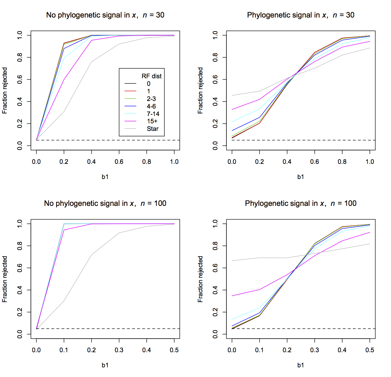
phylolm() (Pagel’s λ model) using a Wald test.As the number of mistakes in the topology of the phylogeny increases, the type I errors and power become qualitatively more similar to the case when phylogenetic signal in the residual errors is ignored (gray line in Fig. 3.10 labelled “Star” given by a LM model). When there is no phylogenetic signal in x, power is lost with increasing numbers of topological mistakes. When there is phylogenetic signal in x, type I errors become more inflated with increasing numbers of mistakes. When n = 30, a single topological mistake (red lines) makes little difference, although even 2-3 topological mistakes can noticeably inflate the type I errors when there is phylogenetic signal in x. The same number of topological mistakes has less effect when n = 100, which is not surprising, because with more species the same number of topological mistakes leaves more of the initial phylogeny intact.
Problems with type I errors and power that we have encountered in this book up to now can be overcome using bootstrapping. To account for uncertainty in the topology of phylogenies, it is necessary to bootstrap over the possible topologies, weighing the topologies according to their likelihoods (Martins 1996). As phylogenies are getting more and more common, and better and better, this issue will hopefully recede. Also, if the topological mistakes are few, they have small impact on type I errors and power. Nonetheless, the issue of topological mistakes in a phylogeny should be recognized and considered in analyses of comparative data.
3.8 Phylogenetic regression for binary data
There are two general approaches for fitting phylogenetic models to binary data. The first uses a logit normal-binomial model in which the normal distribution is multivariate with a covariance given by Brownian motion evolution. This phylogenetic generalize linear mixed model (PGLMM) is similar to the GLMMs discussed in chapters 1 and 2. The second approach is based on logistic regression. Because a discussion of phylogenetic methods for binary data is given in Ives and Garland (2014), I will be brief here.
3.8.1 Binary PGLMM
The structure of the binary PGLMM is like the binary GLMM, but with e having phylogenetic signal given by Brownian motion evolution:
Z = b0 + b1*x + e
p = inv.logit(Z)
Y ~ binom(n, p)
e ~ norm(0, s2*V)
Here, because it is possible for s2 to be zero, there is no need to include a branch-length transform for the covariance matrix V; if there is phylogenetic signal, then s2 will be greater than zero.
Although this model has a relatively simple structure, there are few off-the-shelf methods for fitting it. In the package ape, the function binaryPGLMM() fits this model using a combination of penalized quasi-likelihood and REML (Ives and Helmus 2011); a faster version of binaryPGLMM() written in C++ is in the package phyr. Because it uses quasi-likelihoods, binaryPGLMM() doesn’t give a likelihood, which makes likelihood ratio tests impossible. Nonetheless, it gives inference about the regression coefficients using Wald tests. I also performed a parametric bootstrap test of H0:b1 = 0. Because binaryPGLMM() does not give log likelihoods, I used the following procedure that bootstraps the parameter value of interest (b1) under H0:b1 = 0 rather than the LLR:
- Fit the model to the data and calculate the value of the parameter of interest (in this case, b1).
- Refit the model without the parameter (without x1) and use the resulting parameter values to simulate a large number of datasets.
- Refit the model including the parameter of interest (b1) for each dataset and collect these values.
- The resulting distribution of parameters estimated from the simulated datasets approximates the distribution of the estimator of the parameter under H0:b1 = 0, allowing P-values to be calculated. For a two-tailed test, the P-values are twice the fraction of simulated parameter values that exceed the value estimated from the data with the full model (step i).
The binary PGLMM can also be fit using Bayesian methods, such as in the package MCMCglmm (Hadfield 2010).
3.8.2 Phylogenetic logistic regression
Logistic regression is identical to a binary GLMM when the errors aren’t correlated. Nonetheless, in phylogenetic logistic regression (PLOG) the phylogenetic covariances are incorporated differently from PGLMM. In PLOG models, the value of a binary trait (0 or 1) changes as it evolves up a phylogenetic tree (Ives and Garland 2010), and this can be used to calculate the likelihood. Logistic regression in general gives regression coefficients that are biased upwards; this was seen in figure 2.6 (subsection 2.6.3). A good way to correct for this bias is to apply a penalty to the likelihood function (Firth 1993, Ives and Garland 2010), and PLOG as implemented by phyloglm() use this Firth penalized likelihood. Finally, the effects of the predictors x are added after the evolution up the phylogenetic tree; these changes caused by x occur as an instantaneous switch from 0 to 1, or 1 to 0, depending on the values of x and the regression coefficients.
3.8.3 Type I errors and power
To investigate type I errors and power, I performed a study using a binary PGLMM to simulate data for the cases in which x does not and does have phylogenetic signal (Fig. 3.11). Both the binary PGLMM (binaryPGLMM()) and PLOG (phyloglm()) showed inflated type I errors when x had phylogenetic signal, with PLOG being particularly bad. The inflated type I errors were of course corrected using the bootstrap under H0:b1 = 0. The bootstrapped PGLMM had greater power than the bootstrapped PLOG; this might be the consequence of the data having been simulated using a PGLMM model. Finally, unlike the case of hierarchical data in which LMs and LMMs often performed well on binary data, in this case the continuous PGLS (phylolm()) either had inflated type I errors (when x had no phylogenetic signal) or very low power (when x had phylogenetic signal).
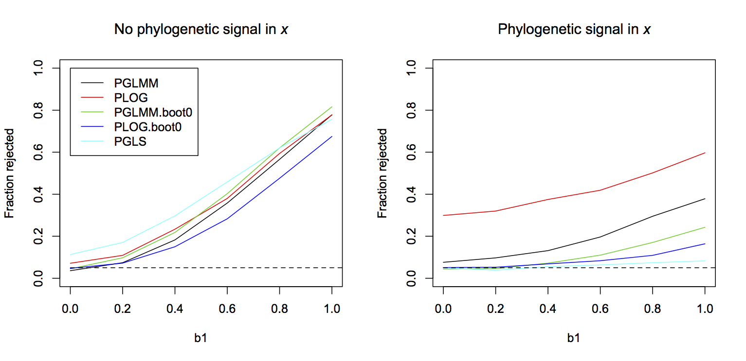
binaryPGLMM()) and PLOG (phyloglm()) using Wald tests, binary PGLMM and PLOG using bootstraps under H0:b1 = 0, and a PGLS (phylolm()) that does not account for the binary nature of the data.Finally, one thing to note about these simulations is that the power of all the methods with proper type I error control was low when there was phylogenetic signal in x, even though the sample size was n = 50, rather than n = 30 as in analyses presented previously for continuous data (Fig. 3.9). This is a reflection of the fact that there is not as much information in binary data as in continuous data, and phylogenetic signal in the residual errors and x compounds this lack of information.
3.9 Summary
- Phylogenetic comparative methods involve models that explicitly include the hypothesis that phylogenetically related species are more likely to have similar trait values. Incorporating branch-length transforms, such as Pagel’s λ and OU transforms, gives a way to test this hypothesis. In regression analyses for phylogenetic data, branch-length transforms should be included to let the data say whether there is phylogenetic signal in the residual errors.
- Estimating the strength of phylogenetic signal involves estimating covariances in the data. Estimating covariances is sometimes harder statistically than estimating regression coefficients, and therefore this requires caution. Also, phylogenetic covariances can take different forms, and therefore you should anticipate that one branch-length transform might fit the data better than others.
- All of the issues that can corrupt results from analyses of hierarchical data also apply to phylogenetic data. In particular, don’t trust the P-values that are reported even from established methods.
- As found for hierarchical data, failing to account for phylogenetic correlation can lead to badly inflated type I errors (false positives). This occurs especially when there is phylogenetic signal in x.
- Most phylogenetic comparative analyses are performed under the assumption that the topology of the phylogeny is correct. When it is not correct, increasing topological mistakes increase the statistical problems that are found when phylogenetic signal is ignored altogether.
- Phylogenetic models can be formulated for binary data. These models experience the same challenges as models for continuous data, with the challenges exacerbated by the lower information content of binary data.
3.10 Exercises
- Construct the right panel of figure 3.8 giving power curves for the detection of phylogenetic signal in simulated data using an OU transform. You can modify the code I provided for the left panel which simulates data using Pagel’s λ transform.
- The parametric bootstrap of H0 for phylogenetic signal (subsection 3.5.3) uses the log likelihood ratio (LLR) as the test statistic. It is also possible to use the phylogenetic signal parameter (λ or α) as the test statistic. This would involve the following: (i) Fit the model to the data and calculate the value of the phylogenetic signal parameter (λ or α). (ii) Refit the model with no phylogenetic signal and use the resulting parameter values to simulate a large number of datasets. (iii) Refit the model including the phylogenetic signal parameter (λ or α) for each dataset and collect these values. (iv) The resulting distribution of λ or α estimated from the simulated datasets approximates the distribution of the estimator of λ or α, allowing P-values to be calculated. Perform this bootstrap and compare the results to the bootstrap of H0 using the LLR.
- In subsection 3.6.1 I showed that, if phylogenetic signal in the residual errors is caused by unmeasured traits with phylogenetic signal, then increasing the number of unmeasured traits doesn’t degrade the phylogenetic signal. In other words, the signals from the unmeasured traits don’t cancel each other out. Perform a simple simulation with three unmeasured traits to show this is true.
3.11 References
Bartoszek K., Pienaar J., Mostad. P., Andersson S. and Hansen T.F. 2012. A phylogenetic comparative method for studying multivariate adaptation. Journal of Theoretical Biology 314:204-215
Blomberg S.P., Garland T. Jr., and Ives A.R. 2003. Testing for phylogenetic signal in comparative data: behavioral traits are more labile. Evolution 57:717-745.
Butler M.A. and King A.A. 2004. Phylogenetic comparative analysis: a modeling approach for adaptive evolution. American Naturalist 164:683-695.
Efron B. and Tibshirani R.J. 1993. An introduction to the bootstrap. Chapman and Hall, New York.
Firth D. 1993. Bias reduction of maximum likelihood estimates. Biometrika 80:27-38.
Hadfield J.D. 2010. MCMC methods for multi-response generalized linear mixed models: the MCMCglmm R package. Journal of Statistical Software 33:1-22.
Hansen T.F. and Orzack S.H. 2005. Assessing current adaptive and phylogenetic inertia explanations of trait evolution: the need for controlled comparisons. Evolution 59:2063-2072.
Ho L.S.T. and Ane C. 2014. A linear-time algorithm for Gaussian and non-Gaussian trait evolution models. Systematic Biology, 63(3):397-408.
Ives A.R., Midford P.E., and Garland T. Jr. 2007. Within-species variation and measurement error in phylogenetic comparative methods. Systematic Biology 56:252-270.
Ives A.R. and Garland T. Jr. 2010. Phylogenetic logistic regression for binary dependent variables. Systematic Biology 59:9-26.
Ives A.R. and Garland T. Jr. 2014. Phylogenetic regression for binary dependent variables. Pages 231-261 in L. Z. Garamszegi, editor. Modern Phylogenetic Comparative Methods and Their Application in Evolutionary Biology. Springer-Verlag, Berlin Heidelberg.
Ives A.R. and Helmus M.R. 2011. Generalized linear mixed models for phylogenetic analyses of community structure. Ecological Monographs 81:511-525.
Martins E.P. 1996. Conducting phylogenetic comparative studies when the phylogeny is not known. Evolution 50:12-22.
Martins E.P. and Hansen T.F. 1997. Phylogenies and the comparative method: A general approach to incorporating phylogenetic information into the analysis of interspecific data. American Naturalist 149:646-667.
Pagel M. 1997. Inferring evolutionary processes from phylogenies. Zoologica Scripta 26:331-348.
Pagel M. 1999. Inferring the historical patterns of biological evolution. Nature 401:877-884.
Paradis E., Claude J. and Strimmer K. 2004. APE: analyses of phylogenetics and evolution in R language. Bioinformatics 20: 289-290
Rangel T.F., Colwell R.K., Graves G.R., Fucikova K., Rahbek C., and Diniz J.A.F. 2015. Phylogenetic uncertainty revisited: Implications for ecological analyses. Evolution 69:1301-1312.
Revell L.J. 2010. Phylogenetic signal and linear regression on species data. Methods in Ecology and Evolution 1:319-329.
Revell L.J. 2012 phytools: An R package for phylogenetic comparative biology (and other things). Methods in Ecology and Evolution 3: 217-223.
Robinson D.F. and Foulds L.R. 1981. Comparison of phylogenetic trees. Mathematical Biosciences 53:131-147.