Chapter 2: Good Statistical Properties
2.1 Introduction
When there are many possible methods for analyzing a dataset, it is necessary to ask which one is best. What properties should you look for in a statistical method? And how should you look? In Chapter 1 I presented a collection of nine methods for analyzing a simple dataset. Some gave the same results, and others didn’t. Which method, and hence which results, should you believe? While you might think that the best method will be the one that incorporates all of the attributes of the data – for the grouse data in particular, this would be both the correlation structure of the residuals and the binomial nature of the data. But this is a mistake. Incorporating all the attributes of the data does not guarantee that the method is best, and just because a method doesn’t have all the attributes of the data doesn’t mean it will perform poorly.
Selecting a good statistical method involves two conceptually distinct issues. First, you want a statistical method that, if it really does properly describe the underlying process that generated your data, gives you the correct information about the data. You need to be aware that you can’t take this for granted. For example, just because the output from a statistical package gives you a P-value of 0.034, you shouldn’t necessarily believe this value. As I’ll show in this chapter, even very standard methods do not give you the correct P-values. On the bright side, these problems with statistical methods are relatively easy to discover and only a little more difficult to correct. Second, you want to know how misleading your statistical results might be if your model doesn’t properly describe the underlying process that generated your data. This second issue is more difficult than the first issue, because you will never really know what the process underlying your data is. Nonetheless, you can at least explore reasonable possibilities for these processes and see how your method performs. Be cautious.
Although these two issues are conceptually distinct, in practice the same approaches can be used to assess each. The approaches involve simulations. For the first issue – checking on the properties of your statistical tests when you assume the model is correct – the simulations are technically referred to as parametric bootstraps. For the second issue – checking on the properties of your statistical tests when you don’t assume the model is correct – the simulations are just simulations. I use simulations a lot, and I am generally skeptical of any result until I have done simulations. In the ecological and evolutionary literature, I’m often surprised to see new methods presented without a battery of simulations to test how they work. In the statistics literature, this would not pass muster.
The chapter starts with a description of the properties of estimators (functions that estimate parameters in a model) that should be used to assess how good they are. It then addresses properties of hypothesis testing involving estimators. Thus, the chapter presents:
| Properties of Estimators |
| Bias |
| Efficiency (Precision) |
| Consistency |
| Properties of Hypothesis Tests |
| Type I errors |
| Power |
I’ll first present these properties using simple Ordinary Least-Squares (OLS) regression with data in which the error terms are independent and identically distributed normal random variables, because this is one of the few cases in which the statistical properties of estimators are correct. I’ll then repeat the investigation for a binary (logistic) regression problem. Finally, I’ll return to the nine methods we applied to the ruffed grouse data in Chapter 1 to try to sort out which method is best.
2.2 Take-homes
- Estimators are functions of random variables that describe your data and have useful properties that lead to estimates of parameters in statistical models. Because they are functions of random variables, they are themselves random variables, and their properties – expectation, variance, behavior as sample sizes increase, etc. – determine the quality of the parameter estimates that they give.
- Don’t trust the P-values that are reported from even standard statistical tests. Test them. If you find a problem with a statistical test, it is often relatively easy to fix the problem using parametric bootstrapping or some other approach.
- As illustrated by the grouse data, failing to account for correlation in your data can lead to badly inflated type I errors (false positives).
- The problem presented by discretely distributed data, or more generally non-normal data, rests mainly in the problem of heteroscedasticity. Often the problem of heteroscedasticity is not that great.
- Hierarchical models, such as LMMs and GLMMs, are sometimes thought to have more statistical power because they use more data. For example, there are more data points in the station-level grouse data than in the route-level data. However, having more data points per se does not increase statistical power, and if you find it does in an analysis you performed, then your statistics are probably wrong. However, if a hierarchical model uses more information from the data, then it can have more power.
2.3 Estimators
Statistical estimators are functions of random variables that have useful properties for fitting a model. To put flesh on that vague definition, suppose you perform an experiment that involves taking n observations. Each observation can be thought of as a draw from a random variable X; a random variable is just a list of possible outcomes of an experiment along with the associated probability of each outcome. For example, suppose your experiment involves flipping a coin; a process like flipping a coin that has two outcomes (heads or tails) is a Bernoulli process. The random variable X describes the possible outcomes – 1 (heads) or 0 (tails) – of each flip and the probability associated with each outcome. The entire experiment of flipping a coin n times could then be represented by the list of random variables (X1, X2, …, Xn). Once you perform the experiment, you have a specific set of outcomes (x1, x2, …, xn) that is a string of 1s and 0s; there are no longer probabilities associated with the outcomes, because you know what the flips produced.
A statistic, as defined by statisticians, is a function of the n random variables (X1, X2, …, Xn). Because it is a function of random variables, a statistic is also a random variable whose mean, variance, and other attributes depend on the n random variables Xi. An estimator is a particular statistic that has useful properties for estimating the parameters of the process X. For example, a possible statistic for estimating the mean number of 1s (heads) from the coin flipping experiment is the estimator W:
W = F(X1, X2, …, Xn) = sum(X1, X2, …, Xn)/n
W is just a function F() that gives the expectation of the random coin flips. Notice that W can’t be computed to give a number until after you have performed the experiment; once you know the heads and tails, the outcome of W is just the average. But when discussing the properties of estimators, it is the properties of the random variable W that are discussed.
In this simple example, W is designed to give estimates of the mean. Estimators can be designed to give estimates of any parameter in a model. For example, there are estimators for slopes (regression coefficients) in regression models, and also estimators for parameters that describe the variances and covariances in hierarchical and phylogenetic models. All of these estimators can be judged by the same criteria.
2.3.1 Maximum Likelihood (ML) estimators
How do you derive a good estimator? One of the most common approaches is to derive the maximum likelihood (ML) estimator. The likelihood is the probability of observing a given set of outcomes of an experiment for specified values of the parameters in a model. The greater the probability of obtaining the observed outcome of the experiment, the better the fit of the model. The ML estimates of the parameters are those values that maximize the likelihood of the observed experimental outcome.
It is relatively easy to derive the ML estimator for the coin-flipping Bernoulli process. Let p be the probability of a heads; to make things interesting, we’ll assume that p might not equal 0.5, because there could be a weighted coin. The parameter of the Bernoulli process is thus p, and p is what we want to estimate. A formal description of the Bernoulli process is
Pr(X=1|p) = p
Pr(X=0|p) = (1 - p)
The first of these expressions states that the probability that the random variable X equals one given that the Bernoulli parameter has value p is p, and the second expression is similar. These two expressions can be collapsed into the probability distribution function f(x|p) defined as the probability that a single trial (flip) gives x = 1 or x = 0, conditioned on the value of the parameter p. Thus,
f(x|p)=x*p + (1 - x)*(1 - p)
You can put in values of x (1 or 0) to see that this expression works. The likelihood of the outcome of the entire experiment of n coin flips is the product of all the probabilities of the individual flips, so
L(x1, x2, …, xn|p) = f(x1|p) f(x2|p) … f(xn|p) = prod(xi*p + (1 - xi)*(1 - p))
where prod is the product taken over all i = 1, 2, …, n. Taking the log to give the log likelihood function, logL, turns the products into sums, which are easier to handle mathematically:
logL(x1, x2, …, xn|p) = sum(log(xi*p + (1 - xi)*(1 - p)))
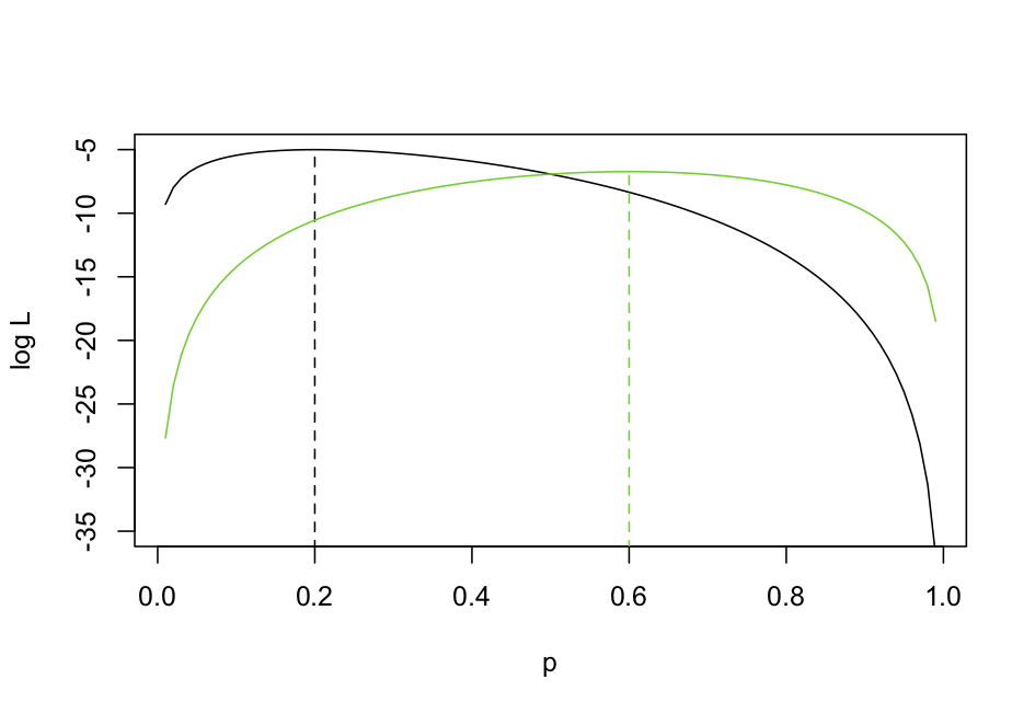
Since xi takes only values 1 and 0, this sum reduces to m*log(p) + (n-m)*log(1-p), where m is the number of 1s in the array x (i.e, the number of successes). To get the ML estimator of p, we want to find an expression that gives the value of p that maximizes the log likelihood (logL). Finding this maximum involves taking the derivative of the logL with respect to p and solving for that p where the derivative is zero (i.e., at the top of the peak in the logL). To illustrate this, figure 2.1 shows the logL for two experiments in which 2/10 (black line) and 6/10 flips (green line) were heads. Reading from the graph you can see in the first case that the ML estimate of p is 0.2, and in the second case it is 0.6. So the ML estimate of p is just the mean number of heads that occurred in the experiment:
W = f(X1, X2, …, Xn) = sum(X1, X2, …, Xn)/n
The ML estimator is what you would guess would be the best estimator based on your intuition. This is a very simple case giving a very simple estimator, but in general ML estimators often are intuitive.
2.4 Properties of estimators
Estimators have a set of properties that measure different aspects of their performance. To illustrate these properties, I’ll use the statistical problem of estimating the slope b1 in the regression model
Y = b0 + b1*x + e
where e is a normal random variable that is independently and identically distributed among samples. Since I want to talk about estimators in general, I will assume that the parameter being estimated is θ. In this problem, θ = b1.
2.4.1 Bias
If an estimator for θ is unbiased, then its expectation equals the actual value of θ:
E[W] = θ
In other words, if you take the values of W from all possible experimental outcomes and weight them by the probability of the outcomes, then this value would be the parameter θ. This is clearly a useful property for an estimator: on average you expect its value to equal the true value of the parameter you are estimating. To test to see if the OLS estimator of b1 is unbiased, I used the function lm() with the following code.
<- 10
b0 <- 1
b1 <- 1
sd.e <- 1
nsims <- 5000
estimate <- data.frame(b0=array(0,dim=nsims), b1=0, b1.P=0, resid2=0, sigma2=0)
for(i in 1:nsims){
x <- rnorm(n=n, mean=0, sd=1)
Y <- b0 + b1*x + rnorm(n=n, mean=0, sd=sd.e)
z <- lm(Y ~ x)
estimate$b0[i] <- z$coef[1]
estimate$b1[i] <- z$coef[2]
estimate$b1.P[i] <- summary(z)$coef[2,4]
estimate$s2.est1[i] <- mean(z$resid^2)
estimate$s2.est2[i] <- mean(z$resid^2)*n/z$df.residual
}
This code first specifies the number of points, n, the parameters b0 and b1 in the model, and the standard deviation of the error e. It then sets the number of simulations, nsim, and defines a data.frame to collect the results, the estimates of b0 and b1, the P-value associated with b1, and two different estimates of the variance of e (used in the next subsection on efficiency). It then iterates through nsim simulations and fits of the model each time.
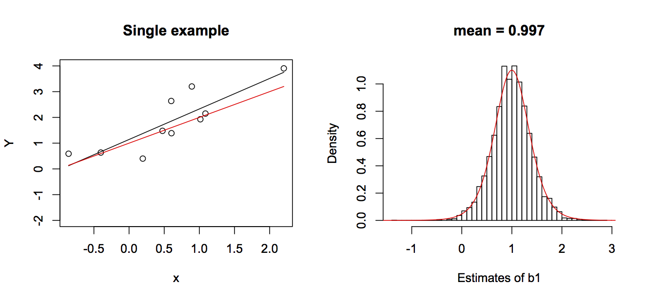
b0 + b1*x in red and the estimated line in black. The right panel gives the nsim = 5000 estimates of b1 and a t-distribution that is theoretically expected to be the distribution of the estimator of b1. The true values for the simulations were b0 = 1 and b1 = 1.The nsim = 5000 estimates of b1 are given in the right panel of figure 2.2. Note that they closely follow a t-distribution parameterized from the model parameters, which is theoretically the distribution of the estimator of b1. This shows that not only is the OLS estimator of b1 unbiased, but the theoretical distribution of the estimator is pretty accurate.
2.4.2 Efficiency (Precision)
An efficient statistic has the lowest variance, that is, the highest precision, of any estimator. Therefore, if We is an efficient estimator, then for any other estimator W,
var[We] ≤ var[W]
The OLS estimator of b1 is the most efficient. In fact, it has been shown by the Gauss–Markov theorem that the OLS estimator of the coefficients of a linear regression model is BLUE, the best linear unbiased estimator, where “best” means the most efficient (Judge et al. 1985). This result doesn’t depend on the error terms being normal, or even identically distributed. But it does require that they be independent and homoscedastic. This property of OLS estimators is why OLS works so well for estimating regression coefficients.
I need to make a brief detour in the discussion right now to avoid a seeming contradiction that you might have spotted. In Chapter 1 (subsection 1.4.1) I introduced the LM and said that it gave good P-values for the regression coefficients even when the data were discrete counts. This is consistent with the discussion of the efficiency of OLS in the last paragraph. However, at the end of Chapter 2 (section 1.6) the regression coefficients estimated from the LM were very different from those estimated from other methods. This is because the LM was applied to transformed data (subsection 1.4.1). The LM is still BLUE, but what it is estimating (the slope of a transformed variable) has a different meaning from a regression coefficient from a GLM (subsections 1.4.2 and 1.4.3). In the GLMs the regression coefficients give estimates of the probabilities p of observing a grouse at a station when transformed through the inv.logit link function. In contrast, the LM does not estimate a value of p. Thus, the LM applied to binomial data can give very good statistical tests for whether there is an association (i.e., whether b1 statistically differs from zero) even though the specific value of the estimate of b1 is difficult to interpret.
I haven’t used simulations to show that the OLS estimator of the regression coefficients is efficient, because this isn’t very interesting; there aren’t any serious contenders. A more interesting case is the estimator of the variance s2 of e. There are two possible estimators of the variance s2. The first is the ML estimator, which is just the mean of the squared residuals. The second is the mean-squared-error (MSE). Specifically,
ML estimator of s2 = (1/n)*sum((Xi - mean(X))2)
MSE estimator of s2 = (1/df)*sum((Xi - mean(X))2)
where df is the degrees of freedom, equal to n minus the number of regression coefficients in the model. Note that the ML and MSE estimates only differ by a constant, with the MSE estimator being (n/df) greater than the ML estimator. The values from these estimators in the simulations are shown in figure 2.3.
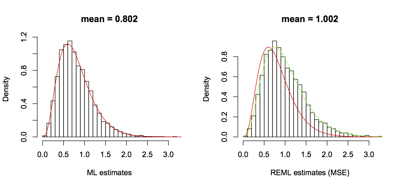
e in the regression model: the ML estimator (left panel) and the MSE estimator (right panel). The red line in both figures gives the theoretical distribution of the ML estimator, and the green line in the right panel gives the theoretical distribution of MSE estimator.ML and MSE estimators show that there is a trade-off in the estimation of s2. The ML estimator has higher efficiency (precision) than the MSE estimator. However, the ML estimator is biased; the expectation of the ML estimator is always below the true value by (n/df). It might seem strange that ML estimator is biased. After all, it is just computed by taking the sample variance of the residuals. The cause for this bias, though, is that in computing the variance of the residuals, the mean value (given by b0 + b1*x) has been estimated by minimizing the residuals (i.e., producing the least squares). In other words, the estimates of b0 and b1 have already been made to minimize the variance of the residuals, so it is not too surprising that the variance of the residuals is lower than the true variance of the errors. I won’t go into the details, but the estimates of the two coefficients b0 and b1 reduce the information available to estimate the variance by the equivalent of two data points (hence the reduction in degrees of freedom by 2) (for details, see Larsen, R.J. and Marx, M.L. 1981).
To put this into a broader context, the MSE is the restricted maximum likelihood (REML) estimator. REML estimators are closely related to ML estimators, but they are specifically designed to estimate the variance components of a model separately from the mean components, which leads to unbiased estimates of the variances (Smyth and Verbyla 1996). In the simple case above, the variance component of the model is just the variance of the residuals, but in hierarchical and phylogenetic models, the variance components also include the covariances and hence the correlated structure of the data. The mean components of the model are the regression coefficients. The separation of mean and variance components in REML often leads to better estimates of both, although this is not always the case.
2.4.3 Consistency
Consistency is the property that the expectation of the estimator of θ becomes arbitrarily close to the true value of θ as the sample size n becomes arbitrarily large. In other words,
E[W] -> θ as n -> ∞
Even if an estimator is biased for small sample sizes, it can still be consistent. For example, the ML estimator of s2 is biased, but as n goes to infinity, it converges to the MSE and the true value of s2 (since n/df converges to one).
It would be nice if not only an estimator were consistent, but also if its precision increased (variance decreased) rapidly with n. Unfortunately, the increase in precision with n is often not as fast as you might think. This is shown by plotting the standard deviation of the OLS estimator for b1 against the sample size (Fig. 2.4). Although the standard deviation drops rapidly initially when the sample sizes are small, the rate of return as sample sizes get larger diminishes, and the standard deviations come nowhere close to zero even for sample sizes of 1000. It is worth making two technical comments. First, the standard deviation of an estimator is the standard error of the estimate. Second, the standard errors of b1 are proportional to the standard deviation of the residual errors. Specifically, I ran these simulations for three values of the standard deviation of the residual errors (sd.e = 1, 2, and 3). Note that the three corresponding standard errors of the estimates of b1 are proportionally the same.
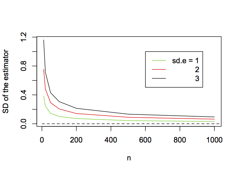
b1 as a function of the sample size for sd.e = 1, 2, and 3.2.5 Hypothesis testing
Hypothesis testing uses the statistical distribution of an estimator (remember, the estimator is a random variable) to infer the probability of the occurrence of a set of observations assuming some null hypothesis is correct. The test then involves claiming that the hypothesis is false if it is deemed sufficiently unlikely (the alpha significance level). This approach contains several arguments of logic.
- There is an underlying process generating the data that could be, at least conceptually, repeated an unlimited number of times. In other words, the experimental observation is described by a random variable X that can be repeatedly sampled.
- Our observation in the experiment is only one of these infinite number of possible realizations.
- We can compare our observation against these realizations and from this assign a probability to what we observed.
- If something is sufficiently unlikely under a null hypothesis, then we are comfortable saying that the hypothesis is false. In doing this, we are conceding that with probability alpha, we have made a mistake, and the null hypothesis is in fact correct even though we say that it is false. But at least we are clear about our grounds for making the call.
In writing the description of hypothesis testing in the last paragraph, I have tried to emphasize the frequentist logic behind it. This contrasts with the logic behind Bayesian statistics, which is distinct from frequentist logic both conceptually and computationally. I’m only bringing up Bayesian statistics here to state that I’m not going to address Bayesian statistics in this book. This isn’t because I have anything against Bayesian statistics. In fact, even though you might hear a lot about how Bayesian and frequentist approaches are fundamentally different and one is superior to the other (with proponents on both sides), I’ve found that most statisticians use one or the other approach depending on the problem. The Bayesian framework leads to algorithms that make it possible to answer statistical problems that would be computationally too hard for frequentist algorithms; therefore, hard problems often pull researchers towards Bayesian statistics. Nonetheless, I have yet to meet a Bayesian statistician who would forgo OLS for estimating parameters for linear regression in favor of a Bayesian approach.
I personally lean towards frequentist approaches because my background is in theoretical ecology, and in theoretical ecology models of real systems are designed and studied often without any attempt to fit them to data. I learned statistics to try to fit theoretical models to data. But with my background in theory, I am used to theoretical models existing before attempting to fit them to data; these theoretical models are thus “reality” that underlie the patterns we observe in nature. This makes me comfortable with the idea that there is some fundamental process, given by a model, underlying the data – the frequentist assumption.
Getting back to hypothesis testing, the two key issues that make a test good are having the correct type I error rates and having good statistical power.
2.5.1 Type I errors
The type I error rate of a statistical test is the probability that the null hypothesis is correct even though it is rejected by the test. Thus, type I errors are false positives. There is nothing wrong with false positives. In fact, they are inevitable and are explicitly set when specifying the alpha significance level of the test. For example, if the alpha significance level is P = 0.05, then there is a 0.05 chance of rejecting the null hypothesis H0 even though it is true. The problem for hypothesis tests involving type I errors is when the alpha significance level you select doesn’t give the actual type I error rate of the test. For example, if you set the alpha significance level at P = 0.05 but the actual chance of rejecting H0 is 0.10, then you run the risk of stating that a result is significant at, say P = 0.045, when in fact the true probability under H0 is 0.090. You would thus be claiming that a result is significant at the alpha significance level of 0.05 when in fact it is not. That would be bad.
The correct control of type I error rates is easy to check. If you simulate data using a model for which H0 is true and fit the model to many simulated datasets, the fraction of simulated datasets for which H0 is rejected should equal the alpha significance level. The code required for doing this for the regression model is very similar to that presented for simulating the distribution of the estimator of b1 to produce figure 2.3 and 2.4, so I won’t reproduce it here (although it is in the R code for this chapter). For parameters in the models, I picked the same values as used in section 2.4.
The results for an alpha significance level of 0.05 and different values of n are
| n | rejected |
| 20 | 0.047 |
| 30 | 0.051 |
| 50 | 0.051 |
| 100 | 0.054 |
There is some variation away from the 0.05, but this is just due to the variation inherent in random simulations. I simulated 10,000 datasets, but more simulations will bring the values closer to 0.05.
2.5.2 Power
Power depends on the chances of rejecting the null hypothesis when in fact it is wrong. It is possible to assess both the power and type I errors of a model by fitting it to simulations as the parameter θ gets increasingly removed from the null hypothesis. Figure 2.5 shows the fraction of 10,000 simulations for which H0:b1 = 0 was rejected at the alpha significance level of 0.05 for values of b1 increasing from zero. The curves for b1 decreasing from zero are the mirror image, so I haven’t shown them. The type I error rate is given when the true value of b1 is 0 (the null hypothesis). If the type I error rates are correct, then the fraction of simulations rejected when b1 = 0 should be 0.05, as they are. The steeper the rejection rate increases as b1 increases, the more powerful the test. The lines show that, as the sample size increases, the power to reject H0 increases too.
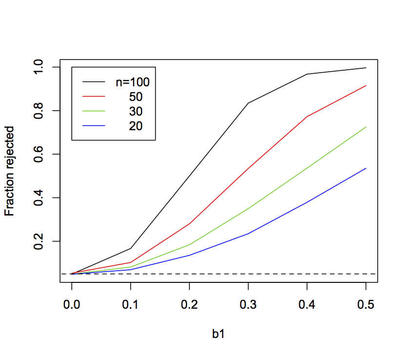
b1 used in the simulations increases from zero. Data were simulated with sample sizes 20, 30, 50, and 100. The horizontal dashed line gives 0.05. In the simulations, b0 = 1 and sd.e = 1, and x was drawn from a normal distribution with mean = 0 and sd = 1.2.6 P-values for binary data
For hypothesis tests of b1 in the linear regression model, the P-values are computing exactly using the fact that the distribution of the estimator of b1 follows a t-distribution. For most methods, however, the exact distribution of the estimator is unknown, and instead an approximation must be used. Two standard approximations are the Wald test and the Likelihood Ratio Test (LRT). I used both of these tests in Chapter 1 with the GLM route-level model (subsection 1.4.2), but here I will go into more detail. I’ll also present two related tests: parametric bootstrapping of the parameter estimate and parametric bootstrapping of the hypothesis test.
To motivate this discussion, I’ll illustrate these different approximations for P-values using a model of binary data with the form
Z = b0 + b1*x1 + b2*x2
p = inv.logit(Z)
Y ~ binom(1, p)
where as before we are focusing on the significance of b1. I’ve added x2 and b2 (where x2 has a norm(0, 1) distribution and b2 = 1.5) because this presents more of a statistical challenge. I simulated the data assuming that x1 and x2 are independent and then fit the data with a binomial GLM. For each fitted GLM I computed the P-values for the null hypothesis H0:b1 = 0 and scored the number of datasets for which H0 was rejected based on four approaches: the Wald test, the LRT, a bootstrap of b1, and a bootstrap of H0. This procedure gives the type I errors (the fraction of simulations rejected at the alpha = 0.05 level) for the case when the true value of b1 = 0. I’ll describe the specific tests later in this section, but I want to start by contrasting their results upfront; this gives you a sense of the problems we face when selecting the best test.
| n | Wald | LRT | Boot(b1) | Boot(H0) | LM | glm.converged |
| 20 | 0.004 | 0.103 | 0.102 | 0.047 | 0.050 | 0.952 |
| 30 | 0.025 | 0.078 | 0.092 | 0.054 | 0.053 | 0.994 |
| 50 | 0.042 | 0.063 | 0.062 | 0.055 | 0.054 | 1.000 |
| 100 | 0.046 | 0.055 | 0.074 | 0.049 | 0.049 | 1.000 |
Obviously, the standard Wald and LRT tests have poor type I error control when sample sizes are small, with the Wald test P-values being far too high (so that rejections occur rarely) and the LRT P-values being far too low (so that rejections occur too frequently). Remember, these are both standard tests, and GLMs are supposed to be appropriate especially for small sample sizes. The parametric bootstrap of the estimated parameter (the column “Boot(b1)”) showed inflated type I errors, with more simulated datasets rejected than the nominal alpha significance level. The parametric bootstrap of the null hypothesis H0 (the column “Boot(H0)”) worked pretty well, giving type I errors of close to 0.05.
For comparison, I also fit a LM to the same data, with the P-value for b1 based on the standard t-test. The LM takes no account of the binary nature of the data, so the actual values of b1 are hard to interpret; for example, the predicted values for Y from the LM can be less than zero or greater than one, even though the values of Y can only be zero or one. Nonetheless, as a test of association (whether b1 is different from zero), the LM did surprisingly well, giving appropriate Type I errors.
There is a small complication in these results, because the function glm() used to fit the GLM didn’t converge for some datasets with small sample sizes. The column labeled “glm.converged” is the fraction of datasets for which convergence was reached. When doing simulations, one could argue for including these cases (lack of convergence could occur with real data) or excluding them (if glm() failed to converge, you would try another method). In this simulation, the P-values either way were not that different, so I only present the results for the cases for which glm() converged.
Finally, there is greater variability in the reported rejection rates for the parametric bootstrap than for the other methods, because I ran fewer simulations. To match the other methods, each of the 10,000 simulations would require 10,000 bootstraps, or a total of 100,000,000 simulations. Therefore, I ran 500 simulations and 1000 bootstrap simulations for each to give the parametric bootstrap of the estimate.
Below I present in more detail the different GLM tests of the null hypothesis H0:b1 = 0 given in the table.
2.6.1 Wald test
The Wald test approximates the standard error of an estimate and then assumes that the estimator is normally distributed with standard deviation equal to the standard error. The Wald test can go wrong in three ways. First, the estimate of the standard error could be wrong. Second, the estimator might not be normally distributed. Third, the estimator could be biased. All three of these problems greatly diminish with large enough sample sizes, but it is generally impossible to guess how large a sample size is large enough. We’ll see the problems with the Wald test approximation when applying the parametric bootstrap (subsection 2.6.3).
2.6.2 Likelihood Ratio Test (LRT)
The LRT is a very general and useful test. It is based on the change in log likelihood between a full model and a reduced model, where the reduced model has one or more parameters missing. For the example, the reduced GLM model used for testing the significance of b1 is the model excluding x1. If x1 is important for the fit of the full model to the data, then there should be a large drop in the logL when x1 is removed, since the data are less likely to be observed. This drop is measured by the log likelihood ratio (LLR), the difference between logLs of full and reduce models. As the sample size increases, 2*LLR approaches a chi-square distribution; for GLMs, 2*LLR is referred to as the deviance. This gives the probability of the change in logL if in fact the reduce model was the true model (i.e., b1 = 0) and hence the statistical test for H0. A particularly useful attribute of the LRT is that more than one parameter can be removed, so joint hypotheses about multiple parameters can be tested. The problem with the test, however, is that the chi-square distribution is only an approximation, and the approximation for our example problem is not very good for even a sample size of 50, as shown in the table above.
2.6.3 Parametric bootstrap of b1
A parametric bootstrap is simple to apply and often very informative; many packages (such as lme4 and boot) provide easy tools to perform a parametric bootstrap. The idea is simple (Efron and Tibshirani 1993):
- Fit the model to the data.
- Using the estimated parameters, simulate a large number of datasets.
- Refit the model to each simulated dataset.
- The resulting distribution of parameters estimated from the simulated datasets approximates the distribution of the estimator, allowing P-values to be calculated.
To show an example with a single dataset, I simulated a dataset with n = 30 and b1 = 1. I fit the model (mod.dat in the code below) that gave an estimated value of b1 = 1.79 (even though the true value was 1; this was not an unusual simulation, though). I then computed the bootstrap P-value:
# Fit dat with the full model
mod.dat <- glm(Y ~ x1 + x2, family = binomial, data=dat)
summary(mod.dat)

# Parametric bootstrap
boot <- data.frame(b1=array(NA,dim=nboot), converge=NA)
dat.boot <- dat
for(i in 1:nboot){
	dat.boot$Y <- simulate(mod.dat)[[1]]
	mod.boot <- glm(Y ~ x1 + x2, family = binomial, data=dat.boot)
	boot$converge[i] <- mod.boot$converge
	boot$b1[i] <- mod.boot$coef[2]
}
# Remove the cases when glm() did not converge
boot <- boot[boot$converge == T,]
pvalue <- 2*min(mean(boot$b1 < 0), mean(boot$b1 > 0))
I used the R function simulate() that takes a model and simulates it for its fitted parameters (which in this case is b1 = 1.79). The simulated data are then refit with a model having the same form as mod.dat. I made the decision only to use bootstrap simulations for which glm() converged. In the bootstrap, the P-value is the proportion of bootstrap values of b1 that extend beyond zero, multiplied by 2 because we are only interested in whether b1 is more extreme than zero regardless of its sign (i.e., a two-tailed test). To explain the code, mean(boot$b1 < 0) is the proportion (mean) of the bootstrapped values of b1 that is less than zero. If the estimate of b1 is greater than zero, then this proportion will be less than 0.5. Therefore, it will be selected by the min() function. This is thus the probability of that the true value of b1 is less than zero, conditioned on the fitted value being greater than zero. Because the fitted value of b1 could have been less than zero, it is necessary to multiply by 2, so that the P-value gives the unconditional probability that the fitted b1 is greater than or less than zero.
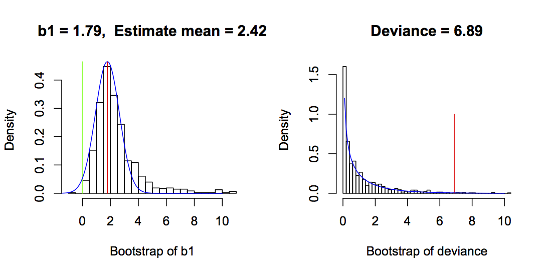
b1 values less than zero; here, P = 0.014. The normal distribution of the estimator of b1 used for the Wald test is given by the blue line, and the P-value from the Wald test is 0.037. The right panel gives the bootstrap values of the deviance (= 2*LLR) for the parametric bootstrap around H0 for the same dataset. The red line is the deviance from the fitted data, and the P-value is 0.011. The green line is at zero. The chi-square distribution from a standard LRT is shown in blue, and the LRT P-value is 0.0086. In both bootstraps, bootstrap datasets for which glm() failed to converge are excluded, and for the parametric bootstrap of b1, values >2.5 times the standard deviation of the estimates are excluded. Other parameters are b0 = 1, b2 = 1.5, the variances of x1 and x2 are 1, and x1 and x2 are independent.The left panel of figure 2.6 gives an example of the bootstrap of b1 and reveals several interesting things about the GLM estimator and the Wald test. First, even though the bootstrap simulations were performed with a model in which b1 = 1.79 (the fitted value), the mean of the bootstrapped estimates was 2.42. This shows that the GLM estimator of b1 is biased upwards. Second, the distribution of the estimator is skewed away from zero. In contrast to the bootstrap estimator of b1, the Wald estimator (blue line) is normal and symmetrical. These differences lead to different P-values, with the parametric bootstrap giving P = 0.002 and the Wald test giving P = 0.037.
These results were generated for a single dataset, yet they are typical of the performance of the bootstrap of b1 and the Wald test. The table at the top of this section shows the rejection rates of the null hypothesis H0:b1 = 0 for a large number of simulated datasets. This table shows that the bootstrap of b1 generally gives P-values that are too low, since the proportion of datasets rejected at the 0.05 level is greater than 5%. It also shows that the Wald P-values are too high, since the proportion of datasets rejected at the 0.05 level is less than 5%. Figure 2.6 is just a single example, and H0:b1 = 0 was rejected by both bootstrap and Wald tests. Nonetheless, the much lower P-value for the bootstrap test of b1 appears to be general for this binary regression model.
2.6.4 Parametric bootstrap of H0
A parametric bootstrap of the null hypothesis H0 is very similar to the parametric bootstrap of the parameter b1, but the data are simulated under H0:
- Fit the model to the data and calculate the deviance (= 2
*LLR) between the full model and the reduced model without b1. - Using the estimated parameters from the reduced model, simulate a large number of datasets.
- Refit both the full and reduced models for each dataset and calculate the deviance.
- The resulting distribution of deviances estimated from the simulated datasets approximates the distribution of the estimator of the deviance, allowing P-values to be calculated.
This is closely related to the LRT, although rather than assume that the deviances are distributed by a chi-square distribution, the distribution of the deviances is bootstrapped.
# Parametric bootstrap of H0
mod.dat <- glm(Y ~ x1 + x2, family = binomial, data=dat)
mod.reduced <- glm(Y ~ x2, family = binomial, data=dat)
LLR.dat <- 2*(logLik(mod.dat) - logLik(mod.reduced))[1]

boot0 <- data.frame(LLR=rep(NA, nboot), converge=NA)
dat.boot <- dat
for(i in 1:nboot){
	dat.boot$Y <- simulate(mod.reduced)[[1]]
	mod.glm <- update(mod.dat, data=dat.boot)
	mod.glm0 <- update(mod.reduced, data=dat.boot)
	boot0$LLR[i] <- 2*(logLik(mod.glm) - logLik(mod.glm0))[1]
	boot0$converge[i] <- mod.boot0$converge
}
# Remove the cases when glm() did not converge
boot0 <- boot0[boot0$converge == T,]
pvalue <- mean(boot0$LLR > LLR.dat)
In figure 2.6, the bootstrapped deviances are similar to the chi-square distribution used in the LRT, although the tail of the bootstrap distribution is wider and longer. This gives the bootstrap P = 0.011, while for the LRT the P-value is 0.0086. The lower P-value for the LRT is consistent with the table at the beginning of this section, in which the LRT gave inflated type I error rates. The good performance of the parametric bootstrap of H0 can be understood by considering the distribution of the estimates of b1. While these estimates aren’t used for the significance test, the distribution of the estimates is symmetrical and therefore necessarily unbiased because the bootstrap simulations are performed under H0:b1 = 0. The better behavior of the estimator of b1 under H0 explains the better performance of the parametric bootstrap of H0 compared to the parametric bootstrap of the parameter b1 (subsection 2.6.3).
2.6.5 Why did the LM do so well?
I included the LM in the table at the top of this section to show that in fact it does as well or better than any of the other methods, at least in terms of type I error. In some respects, this is not surprising. As I discussed in subsection 2.4.2, the OLS estimator of LMs is BLUE (best linear unbiased estimator), provided the errors are independent and homoscedastic. They are independent in the binary model analyzed here, but are they homoscedastic? If this were a univariate binary regression model with only x1, then under the null hypothesis that b1 = 0, they will be homoscedastic, because under H0 there is no variation in the mean, which is determined by b0. With no variation in the mean, there is also no variation in the variance. In the model, however, there is x2. If x2 changes the mean (b2 ≠ 0), then this will generate heteroscedasticity, but if x1 and x2 are independent, then this heteroscedasticity will have no effect on type I errors for the estimate of b1, because the differences in the variances among errors will be independent of x1. However, I would anticipate a problem with heteroscedasticity for the case when b2 > 0, and x1 and x2 are correlated, because this should produce a gradient in heteroscedasticity of residuals across values of x1. But it turns out for the binary model that even this case does not degrade the good type I error control. Figure 2.7 shows an example of the distribution of residuals with b1 = 1.5 and a covariance of 0.8 between x1 and x2 using a large enough sample size (n = 1000) to allow assessment of heteroscedasticity of the residuals. There is some, with the variance in residuals decreasing with increasing b1. However, it is not great, and apparently not great enough to badly degrade the type I error control of the LM. For other families of distributions used in GLMs, such as the binomial distribution with n ≥ 2 or the Poisson distribution, this might not be the case, and the combination of b2 > 0 and correlation between x1 and x2 could cause inflated type I errors; I’ve left this as an exercise. At least for the binary case – the case that is least like continuous data – the LM does well.
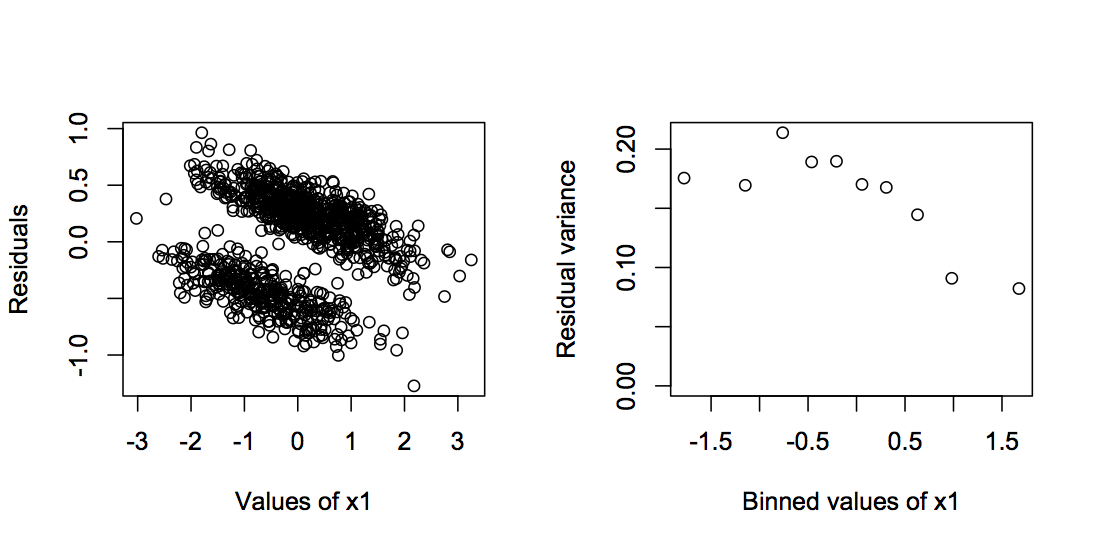
n = 1000, b0 = 1, b1 = 0, b2 = 1.5, the variances of x1 and x2, var.x = 1, and the covariance between x1 and x2, cov.x = 0.8.2.6.6 Power in fitting the binary data
The power and type I error rates of the four methods for computing P-values from the binary GLM, plus the LM, can be shown (as in figure 2.5) by plotting the rejection rate of simulated datasets against the value of b1 used in the simulations. Figure 2.8 repeats the results that the Wald test gives deflated type I errors, the LRT and parametric bootstrap of b1 give inflated type I errors, and the parametric bootstrap of H0 and the LM give pretty good type I errors. Type I errors have to be correct before it makes sense to investigate power; otherwise, you could always increase the power of your test by increasing the type I error rate. Therefore, I shouldn’t really show the power curves for the LRT and parametric bootstrap of b1. Nonetheless, I have. The power of the parametric bootstrap of H0 and the LM are almost identical. Not surprisingly given its lower type I error rates, the Wald test has less power. And while the LRT and parametric bootstrap of b1 appear to have higher power, they shouldn’t be used in the first place due to inflated type I errors.
I left out one good method for performing regressions on binary data: logistic regression using a penalized likelihood function proposed by Firth (1993). I have left you to explore this as an exercise.
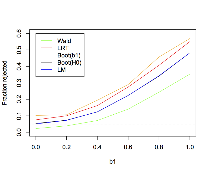
n = 30, b0 = 1, b2 = 1.5, var.x = 1, and cov.x = 0.2.7 Example data: grouse
We are finally in position to return to the grouse data to ask which methods for analyzing the data are best. For this, I will assess the methods based on their type I error control and their power, using the same approach I used for the linear regression model and binary GLM investigated in the last two sections. As a reminder, here are the different methods and the results they give for the effect of wind speed (WIND_MEAN in the route-level methods and WIND in the station-level methods) on the observed abundance of grouse:
| Aggregated data (site-level) | estimate | P-value |
| LM | -0.138 | 0.0436 |
| GLM(binomial) | -0.494 | 0.0082 |
| GLM(quasibinomial) | -0.495 | 0.0992 |
| GLMM | -0.720 | 0.0496 |
| Hierarchical data (plot-level) | ||
| LM | -0.056 | 0.0026 |
| GLM | -0.388 | 0.0030 |
| GLM(ROUTE as a factor) | -0.423 | 0.0534 |
| GLMM | -0.459 | 0.0108 |
| LMM | -0.050 | 0.0114 |
There is an important distinction between the assessment of the approximations used to calculate P-values in the linear regression (Fig. 2.5) and binary GLM (Fig. 2.7) versus the assessment of the methods used to analyze the grouse data presented below. In the assessments of linear regression and binary GLM, the methods used for computing the P-values were assessed using simulations of the same model. Therefore, these gave assessments of the approximations used to compute P-values under the assumption that the models were correct. For the grouse data, I’m going to simulate the data with the station-level GLMM and fit models for all nine different methods. This procedure assesses the methods in their ability to fit data from the data simulated from a different model. Therefore, there is the explicit assumption that the simulation model is correct. In most situations, we wouldn’t know if the station-level GLMM does in fact describe the process that underlies the real grouse data. In this particular case, however, I do in fact know that the station-level GLMM describes the process that underlies the “real” grouse data, since I used it to simulate the “real” grouse data. But I also know that the station-level GLMM does fit the real grouse data well.
2.7.1 Simulating the grouse data
It is convenient to write a function to simulate the station-level grouse data:
<- function (d, b0, b1, sd) {
# This is the inverse logit function
inv.logit <- function(x){
1/(1 + exp(-x))
}
d.sim.Y <- array(-1, dim=dim(d)[1])
for(i in levels(d$ROUTE)){
dd <- d[d$ROUTE == i,]
nn <- dim(dd)[1]
Z <- b0 + b1*dd$WIND + rnorm(n=1, mean=0, sd=sd)
p <- inv.logit(Z)
d.sim.Y[d$ROUTE == i] <- rbinom(n=nn, size=1, prob=p)
}
return(d.sim.Y)
}
This function has the three parameters, b0, b1, and sd as inputs, along with the entire dataset d that contains the station-level data. The dataset d is included, because the simulations use the same numbers for stations in each route, and the same values of WIND at each station, as the real data.
2.7.2 Power curves for the grouse data
Figure 2.9 shows the fraction of simulation datasets for which the null hypothesis H0:b1 = 0 is rejected by the nine methods as a function of the value of b1 in the simulations. Because estimates of b1 in the data were negative, I simulated b1 over negative values. For the route-level data, the binomial GLM has badly inflated type I errors. As described in subsection 1.4.5, this occurs because the binomial GLM constrains the variance to equal the mean during model fitting and estimation. When greater-than-binomial variance is allowed, in either the quasibinomial GLM or the logit normal-binomial GLMM, type I errors are much better controlled, although the GLMM still has slightly inflated type I errors. The LM has good type I error control although has lower power. This result of LMs having reasonable type I error control but lower power is common (Ives 2015).
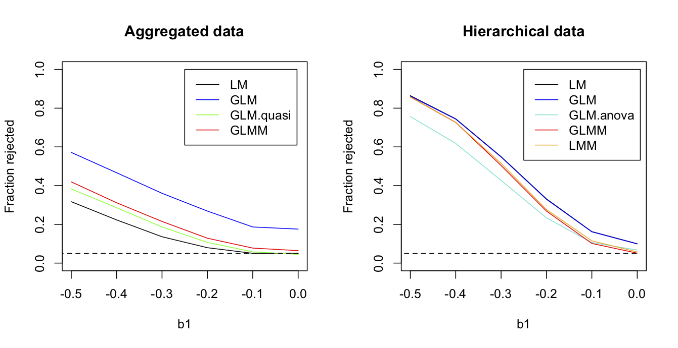
b0 = -1.063, b1 = -0.406, and sd.route = 1.07.Turning to the station-level data, the LM and GLM that don’t account for the correlated structure of the data (stations in the same route having similar grouse abundances) both have inflated type I errors. This is a very common result and is a key reason for accounting for correlated residuals in statistical analyses. The three methods that account for the correlated structure of the data, the LMM and GLMM have pretty good type I error control. The GLM.anova is the GLM in which routes are treated as categorical fixed effects; although GLM.anova has acceptable type I error control, it has lower power. As described in subsection 1.5.4, this likely occurs because no grouse were observed in 22 of the 50 routes, and information from these routes would be absorbed with the route factors and therefore ignored, rather than be used for inference about the effects of WIND.
2.7.3 Do hierarchical methods have more power?
Perhaps the most striking pattern in figure 2.9 is the greater power of the station-level methods in comparison to the route-level methods. Since the station-level methods use datasets with many more points (372 vs. 50), this is not surprising, right? Wrong. The reason for the increased power of the station-level methods is that they use more information, specifically the station-level information about wind speed taken during each station-level observation.
To show that the station-level methods have more power because they have more information, rather than because they have more points, I leveled the playing field by removing the station-level information about wind speed. Specifically, for the station-level analyses I kept everything exactly the same except rather than use the values of WIND measured at each station, instead I assigned the route-level value of MEAN_WIND to all stations within the same route. Thus, the number of data points (372) in the station-level data remained the same, but these points provided no more information about wind speed than the route-level mean. In this case (Fig. 2.10), the powers of the GLMM and LMM applied to the station-level data are almost identical to the powers of the quasibinomial GLM and logit normal-binomial GLMM applied to the route-level data. This is exactly as it should be. If the correlation structure of the data is correctly accounted for, and if the information available from the predictor variables is the same, then analyses of aggregated data should give the same result as analyses of the hierarchical data. If not, your analyses are wrong, since hierarchical models can’t make information from nothing. But comparison with the GLM.anova shows that they can stop you from losing information. The GLM.anova has little power, a consequences of the information lost when it fails to use information from the 22 routes in which no grouse were observed.
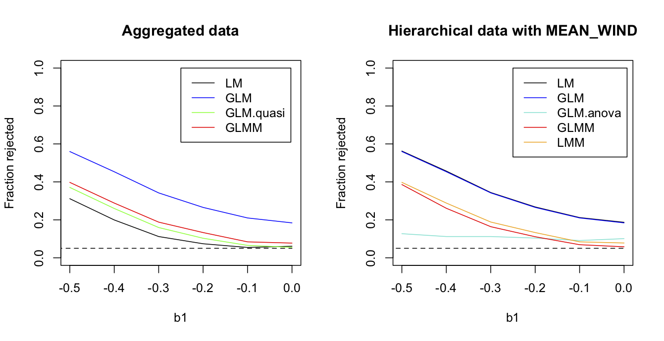
MEAN_WIND is used for all stations within the same route, the fraction of simulations rejected by four methods used to analyze route-level data (left panel) and the five methods used with the station-level data (right panel). Parameter values used to simulation data are b0 = -1.063, b1 = -0.406, and sd.route = 1.07.2.8 Summary
- Estimators are functions of random variables that describe your data and have useful properties that lead to estimates of parameters in statistical models. A good estimator should have an expectation equal to the true value of the parameter it estimates (lack of bias). A good estimator should have high efficiency (high precision or low variance). And a good estimator should be consistent, converging to the true value of a parameter as the sample size increases.
- Even standard statistical tests (except those from OLS) use approximations to compute P-values, and these approximations are prone to poor results when sample sizes are small. You should therefore test them. If you find a problem with a statistical test, it is often relatively easy to use parametric bootstrapping of the null hypothesis to give accurate P-values.
- Failing to account for correlation in your data can lead to badly inflated type I errors (false positives). This was shown with the grouse data, but is a common result.
- The problem presented by discretely distributed data, or more generally non-normal data, rests mainly in the problem of heteroscedasticity. Often the problem of heteroscedasticity is not that great, so linear models are often a robust choice when all that is wanted is a test for whether a relationship is statistically significant. To simulate discrete data, however, it is necessary to fit a GLM or GLMM.
- Hierarchical models, such as LMMs and GLMMs, are sometimes thought to have more statistical power because they use more data. However, having more data points per se does not increase statistical power, and if you find it does, then your statistics are probably wrong. However, if a hierarchical model uses more information in the data, then it can have more power.
2.9 Exercises
- As discussed in subsection 2.6.5, the LM should give good type I errors even when applied to binary data, provided the residuals are homoscedastic. This will be true for the simplest case of only a single predictor (independent) variable, because under the null hypothesis H0:b1 = 0, the residuals will be homoscedastic (since the predicted values for all points are the same). However, if there is a second predictor variable that is correlated to the first, then under the null hypothesis H0:b1 = 0 the residuals will not be homoscedastic. This could generate incorrect type I errors for the LM. In the simulations of binary data, this didn’t seem to cause problems with type I error for the LM (section 2.6). For this exercise, investigate this problem for binomial data with more than two (0 or 1) outcomes. You can modify the code from section 2.6 for this.
- When analyzing the binary regression model, I left out one of the best methods: logistic regression using a Firth correction. I won’t go into details to explain how logistic regression with a Firth correction works, but the basic idea is to fit the regression using ML while penalizing the likelihood so that it doesn’t show (as much) bias as the binomial glm. To see how logistic regression with a Firth correction performs, use the function logistf() in the package {logistf} to produce the same power figure as in Fig. 2.8 (subsection 2.6.6). Don’t bother including the bootstraps, since they take more time. You can still compare how well logistf() does compared to the other methods, since the LM performed the same as the bootstrap of H0. For the simulations, you fit logistf() using the syntax
mod.logistf <- logistf(Y ~ x1 + x2). You can then extract the P-value forx1withmod.logistf$prob[2]. - As an exercise, produce figure 2.10 showing the power curves for the grouse data assuming that the station-level values of
WINDare given byMEAN_WINDfor all stations within the same route. This can be done easily by modifying the code provided for making figure 2.9.
2.10 References
Efron B. and Tibshirani R.J. 1993. An introduction to the bootstrap. Chapman and Hall, New York.
Firth D. 1993. Bias reduction of maximum likelihood estimates. Biometrika 80:27-38.
Ives A.R. 2015. For testing the significance of regression coefficients, go ahead and log-transform count data. Methods in Ecology and Evolution, 6:828-835.
Judge G.G., Griffiths W.E., Hill R.C., Lutkepohl H, and Lee T.-C. 1985. The theory and practice of econometrics. Second edition. John Wiley and Sons, New York.
Larsen R.J. and Marx M.L. 1981. An introduction to mathematical statistics and its applications. Inc., Englewood Cliffs, N. J, Prentice-Hall.
Smyth G.K. and Verbyla A.P. 1996. A conditional likelihood approach to residual maximum likelihood estimation in generalized linear models. Journal of the Royal Statistical Society Series B-Methodological 58:565-572.