Deep Learning Using Deeplearning4j
In the last ten years Deep Learning has been so successful for solving difficult problems in areas like image understanding and natural language processing (NLP) that many people now equate Deep Learning with AI. While I think this is a false equivalence, I have often used both plain old-fashioned neural networks and Deep Learning models in my work. In this chapter we implement a fairly simple feed forward using the general purpose Deeplearning4j (DL4J) library. I implement neural networks “from scratch” in Java and Common Lisp in other books that you can read free online at https://leanpub.com/u/markwatson.
One limitation of conventional back propagation neural networks is that they are limited to the number of neuron layers that can be efficiently trained (the vanishing gradients problem).
Deep learning uses computational improvements to mitigate the vanishing gradient problem like using ReLu activation functions rather than the more traditional Sigmoid function, and networks called “skip connections” where some layers are initially turned off with connections skipping to the next active layer.
Modern deep learning frameworks like DeepLearning4j, TensorFlow, and PyTorch are easy to use and efficient. We use DeepLearning4j in this chapter because it is written in Java and easy to use with Clojure. In a later chapter we will use the Clojure library libpython-clj to access other deep learning-based tools like the Hugging Face Transformer models for question answering systems as well as the spaCy Python library for NLP.
I have used GAN (generative adversarial networks) models for synthesizing numeric spreadsheet data, LSTM (long short term memory) models to synthesize highly structured text data like nested JSON, and for NLP (natural language processing). Several of my 55 US patents use neural network and Deep Learning technology.
The Deeplearning4j.org Java library supports many neural network algorithms. We will look at one simple example so you will feel comfortable integrating Deeplearning4j with your Clojure projects, and a later optional-reading section details other available types of models. Note that I will often refer to Deeplearning4j as DL4J.
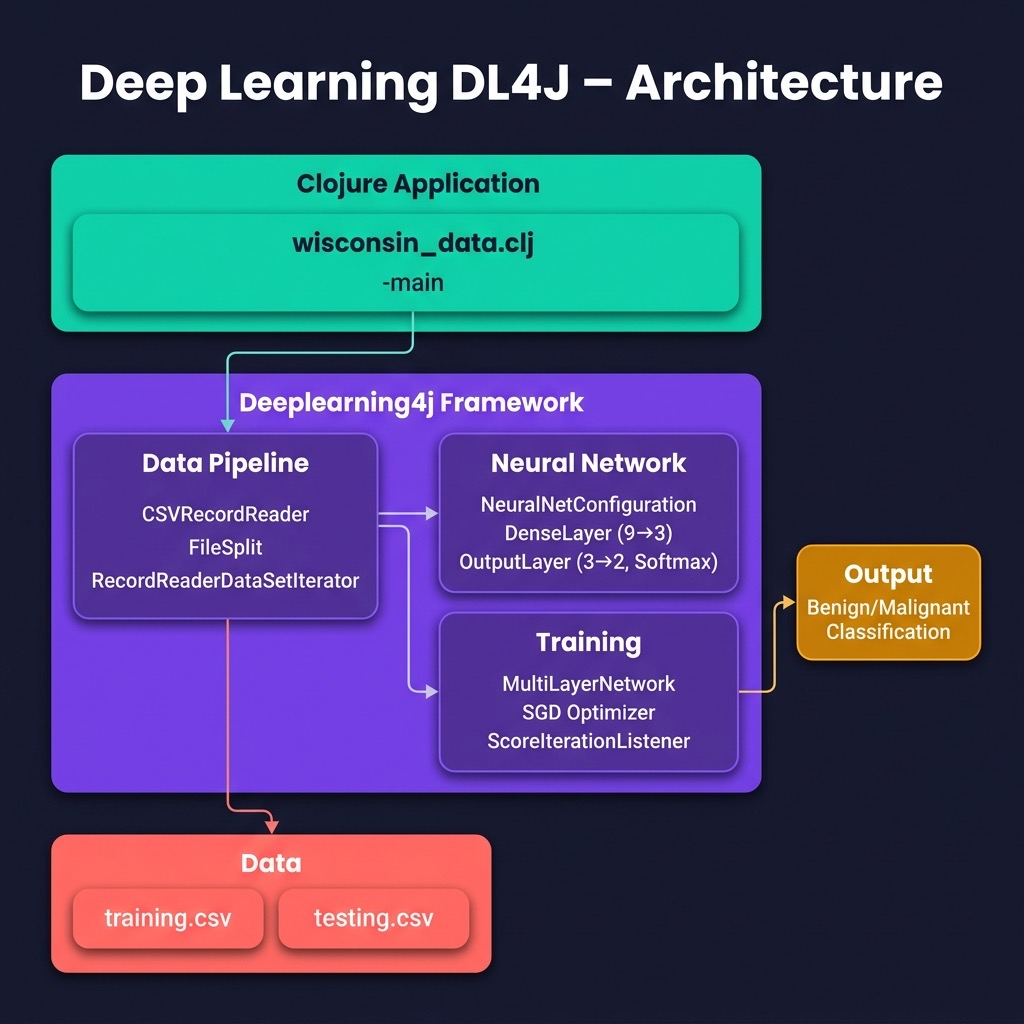
We start with a simple example of a feed forward network using the same University of Wisconsin cancer database that we will also use later in the chapter on anomaly detection.
There is a separate repository of DL4J examples that you might want to look at since any of these Java examples that look useful for your projects can be used in Clojure using the example here to get started.
Feed Forward Classification Networks
Feed forward classification networks are a type of deep neural network that can contain multiple hidden neuron layers. In the example here the adjacent layers are fully connected (all neurons in adjacent layers are connected). The DL4J library is written to scale to large problems and to use GPUs if you have them available.
In general, simpler network architectures that can solve a problem are better than unnecessarily complicated architectures. You can start with simple architectures and add layers, different layer types, and parallel models as needed. For feed forward networks model complexity has two dimensions: the numbers of neurons in hidden layers, and the number of hidden layers. If you put too many neurons in hidden layers then the training data is effectively memorized and this will hurt performance on data samples not used in training (referred to as out of sample data). In practice, I “starve the network” by reducing the number of hidden neurons until the model has reduced accuracy on independent test data. Then I slightly increase the number of neurons in hidden layers. This technique helps avoid models simply memorizing training data (the over fitting problem).
Our example here reads the University of Wisconsin cancer training and testing data sets (lines 37-53), creates a model (lines 53-79), trains it (line 81) and tests it (lines 82-94).
You can increase the number of hidden units per layer in line 23 (something that you might do for more complex problems). To add a hidden layer you can repeat lines 68-75 (and incrementing the layer index from 1 to 2). Note that in this example, we are mostly working with Java data types, not Clojure types. In a later chapter that uses the Jena RDF/SPARQL library, we convert Java values to Clojure values.
 1 (ns deeplearning-dl4j-clj.wisconsin-data
 2   (:import [org.datavec.api.split FileSplit]
 3            [org.deeplearning4j.datasets.datavec
 4             RecordReaderDataSetIterator]
 5            [org.datavec.api.records.reader.impl.csv
 6             CSVRecordReader]
 7            [org.deeplearning4j.nn.conf
 8             NeuralNetConfiguration$Builder]
 9            [org.deeplearning4j.nn.conf.layers
10             OutputLayer$Builder DenseLayer$Builder]
11            [org.deeplearning4j.nn.weights WeightInit]
12            [org.nd4j.linalg.activations Activation]
13            [org.nd4j.linalg.lossfunctions
14             LossFunctions$LossFunction]
15            [org.deeplearning4j.optimize.listeners
16             ScoreIterationListener]
17            [org.deeplearning4j.nn.multilayer
18             MultiLayerNetwork]
19            [java.io File]
20            [org.nd4j.linalg.learning.config Adam Sgd
21             AdaDelta AdaGrad AdaMax Nadam NoOp]))
22
23 (def numHidden 3)
24 (def numOutputs 1)
25 (def batchSize 64)
26
27 (def initial-seed (long 33117))
28
29 (def numInputs 9)
30 (def labelIndex 9)
31 (def numClasses 2)
32
33
34 (defn -main
35   "Using DL4J with Wisconsin data"
36   [& args]
37   (let [recordReader (new CSVRecordReader)
38         _ (. recordReader
39             initialize
40             (new FileSplit
41              (new File "data/", "training.csv")))
42         trainIter
43         (new RecordReaderDataSetIterator
44           recordReader batchSize labelIndex numClasses)
45         recordReaderTest (new CSVRecordReader)
46         _ (. recordReaderTest
47             initialize
48              (new FileSplit
49               (new File "data/", "testing.csv")))
50         testIter
51         (new RecordReaderDataSetIterator
52            recordReaderTest batchSize labelIndex
53            numClasses)
54         conf (->
55                (new NeuralNetConfiguration$Builder)
56                (.seed initial-seed)
57                (.activation Activation/TANH)
58                (.weightInit (WeightInit/XAVIER))
59                (.updater (new Sgd 0.1))
60                (.l2 1e-4)
61                (.list)
62                (.layer
63                  0,
64                  (-> (new DenseLayer$Builder)
65                      (.nIn numInputs)
66                      (.nOut numHidden)
67                      (.build)))
68                (.layer
69                  1,
70                  (-> (new OutputLayer$Builder
71                        LossFunctions$LossFunction/MCXENT)
72                      (.nIn numHidden)
73                      (.nOut numClasses)
74                      (.activation Activation/SOFTMAX)
75                      (.build)))
76                (.build))
77         model (new MultiLayerNetwork conf)
78         score-listener (ScoreIterationListener. 100)]
79     (. model init)
80     (. model setListeners (list score-listener))
81     (. model fit trainIter 10)
82     (while (. testIter hasNext)
83       (let [ds (. testIter next)
84             features (. ds getFeatures)
85             labels (. ds getLabels)
86             predicted (. model output features false)]
87         ;; 26 test samples in data/testing.csv:
88         (doseq [i (range 0 52 2)]
89           (println
90             "desired output: [" (. labels getDouble i)
91             (. labels getDouble (+ i 1)) "]"
92             "predicted output: ["
93             (. predicted getDouble i)
94             (. predicted getDouble (+ i 1)) "]"))))))
Notice that we have separate training and testing data sets. It is very important to not use training data for testing because performance on recognizing training data should always be good assuming that you have enough memory capacity in a network (i.e., enough hidden units and enough neurons in each hidden layer).
The following program output shows the target (correct output) and the output predicted by the trained model:
This is a simple example but is hopefully sufficient to get you started if you want to use DL4J in your Clojure projects. An alternative approach would be writing your model code in Java and embedding the Java code in your Clojure projects - we will see examples of this in later chapters.
Optional Material: Documentation for Other Types of DeepLearning4J Built-in Layers
The documentation for the built-in layer classes in DL4J is probably more than you need for now so let’s review the most other types of layers that I sometimes use. In the simple example we used in the last section we used two types of layers:
- org.deeplearning4j.nn.conf.layers.DenseLayer - maintains connections to all neurons in the previous and next layer, or it is “fully connected.”
- org.deeplearning4j.nn.conf.layers.OutputLayer - has built-in behavior for starting the back propagation calculations back through previous layers.
As you build more deep learning enabled applications, depending on what requirements you have, you will likely need to use at least some of the following Dl4J layer classes:
- org.deeplearning4j.nn.conf.layers.AutoEncoder - often used to remove noise from data. Autoencoders work by making the target training output values equal to the input training values while reducing the number of neurons in the AutoEncoding layer. The layer learns a concise representation of data, or “generalizes” data by learning which features are important.
- org.deeplearning4j.nn.conf.layers.CapsuleLayer - Capsule networks are an attempt to be more efficient versions of convolutional models. Convolutional networks discard position information of detected features while capsule models maintain and use this information.
- org.deeplearning4j.nn.conf.layers.Convolution1D - one-dimensional convolutional layers learn one-dimensional feature detectors. Trained layers learn to recognize features but discard the information of where the feature is located. These are often used for data input streams like signal data and word tokens in natural language processing.
- org.deeplearning4j.nn.conf.layers.Convolution2D - two-dimensional convolutional layers learn two-dimensional feature detectors. Trained layers learn to recognize features but discard the information of where the feature is located. These are often used for recognizing if a type of object appears inside a picture. Note that features, for example, representing a nose or a mouth, are recognized but their location in an input picture does not matter. For example, you could cut up an image of someone’s face, moving the ears to the picture center, the mouth to the upper left corner, etc., and the picture would still be predicted to contain a face with some probability because using soft max output layers produces class labels that can be interpreted as probabilities since the values over all output classes sum to the value 1.
- org.deeplearning4j.nn.conf.layers.EmbeddingLayer - embedding layers are used to transform input data into integer data. My most frequent use of embedding layers is word embedding where each word in training data is assigned an integer value. This data can be “one hot encoded” and in the case of processing words, if there are 5000 unique words in the training data for a classifier, then the embedding layer would have 5001 neurons, one for each word and one to represent all words not in the training data. If the word index (indexing is zero-based) is, for example 117, then the activation value for neuron at index 117 is set to one and all others in the layer are set to zero.
- org.deeplearning4j.nn.conf.layers.FeedForwardLayer - this is a super class for most specialized types of feed forward layers so reading through the class reference is recommended.
- org.deeplearning4j.nn.conf.layers.DropoutLayer - dropout layers are very useful for preventing learning new input patterns from making the network forget previously learned patterns. For each training batch, some fraction of neurons in a dropout layer are turned off and don’t update their weights during a training batch cycle. The development of using dropout was key historically for getting deep learning networks to work with many layers and large amounts of training data.
- org.deeplearning4j.nn.conf.layers.LSTM - LSTM layers are used to extend the temporal memory of what a layer can remember. LSTM are a refinement of RNN models that use an input window to pass through a data stream and the RNN model can only use what is inside this temporal sampling window.
- org.deeplearning4j.nn.conf.layers.Pooling1D - a one-dimensional pooling layer transforms a longer input to a shorter output by downsampling, i.e., there are fewer output connections than input connections.
- org.deeplearning4j.nn.conf.layers.Pooling2D - a two-dimensional pooling layer transforms a larger two-dimensional array of data input to a smaller output two-dimensional array by downsampling.
Deep Learning Wrap Up
I first used neural networks in the late 1980s for phoneme (speech) recognition, specifically using time delay neural networks and I gave a talk about it at IEEE First Annual International Conference on Neural Networks San Diego, California June 21-24, 1987. In the following year I wrote the Backpropagation neural network code that my company used in a bomb detector that we built for the FAA. Back then, neural networks were not widely accepted but in the present time Google, Microsoft, and many other companies are using deep learning for a wide range of practical problems. Exciting work is also being done in the field of natural language processing.
Later we will look at an example calling directly out to Python code using the libpython-clj library to use the spaCy natural language processing library. You can also use the libpython-clj library to access libraries like TensorFlow, PyTorch, etc. in your Clojure applications.