Two: Jeff Hawkins’ Theory of the Neocortex

Hierarchical Temporal Memory and the Cortical Learning Algorithm

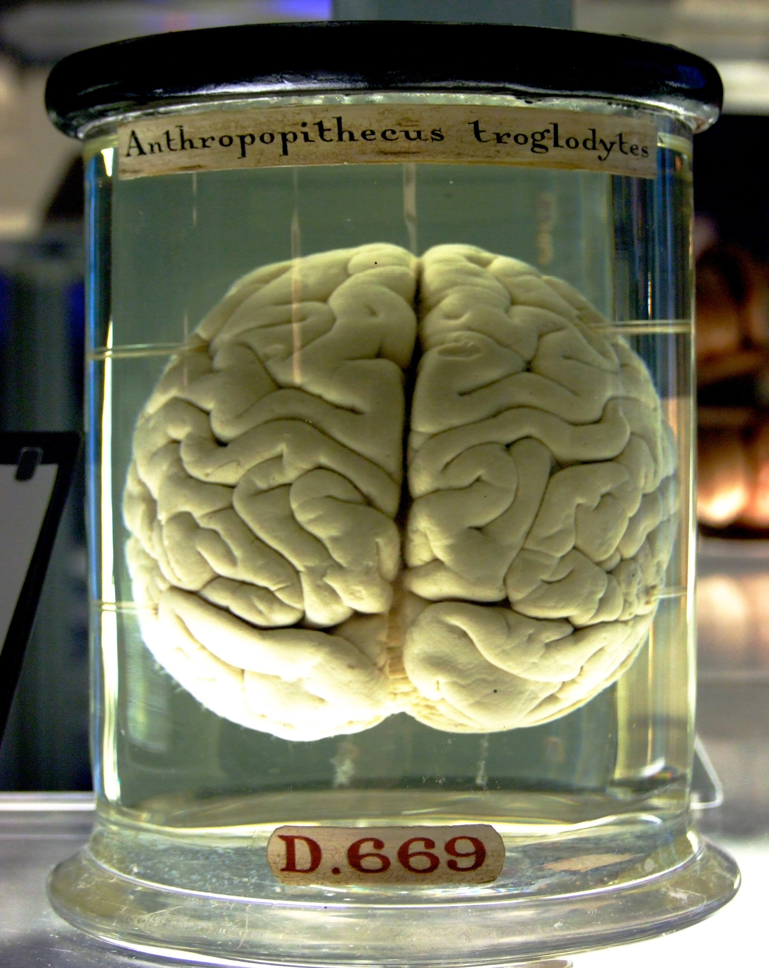
A chimpanzee brain preserved in a jar

A Little Neuroscience Primer

Brain, n.: an apparatus with which we think we think. > Ambrose Bierce, The Devil’s Dictionary

The seat of intelligence is the neocortex (literally “new bark” in Latin) which is the crinkly surface of your brain. This latest addition to the animal brain is only found in mammals, and we have the biggest one of all. The neocortex is crumpled up so that it fits inside the skull; in fact it’s a large surface about the size of a dinner napkin, and has a thickness of about 2mm. The neocortex contains about 60 billion neurons (“brain cells” or “grey matter” - the surface of the brain) which form trillions of connections among themselves (“white matter”, much of which is underneath the crumpled surface) in such a way as to create what we know as intelligence.

Clearly, the neocortex is some kind of computer, in the sense that it is an organ for handling information. But its structure is completely unlike a computer – it has no separate pieces for logic, memory, and input-output. Instead, it is arranged in a hierarchy of patches, or regions, like the staffs and units in an army. At the bottom of the hierarchy, regions of neurons are connected to the world outside the brain via millions of sensory and motor nerves.

Each region takes information from below it, does something with that information, and passes the results up the chain of command. Each region also takes orders of some sort from higher-ups, does something with those orders and passes on, or distributes, more detailed orders to regions below it. Somewhere during this process, the brain forms memories which are related to all this information passing up and down.

The following diagram shows the hierarchy of the macaque monkey’s brain, the part which processes visual information from the eyes. Note that each line in the diagram is more like a big cable, containing hundreds, thousands, or even millions of individual connections between regions.

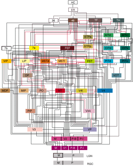
Visual hierarchy of the macaque

Within this hierarchy, each region is remarkably similar in structure. Every region seems to be doing the same thing in the same way as all the others. If you look closely at practically any small piece of neocortex, you’ll see the same pattern again and again, as shown below.

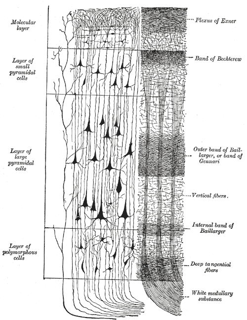
Drawing showing layer structure

As you see in this drawing from Gray’s Anatomy (1918!), neurons are organised vertically in columns, and each column appears to be divided into a number of layers (usually 5 or 6), each of which contains its own “type” of neuron. In addition to what you see here, there are huge numbers of horizontal connections between neighbouring columns; these connections, in fact, add up to almost 90% of all connections in the neocortex.

Two important facts may be observed at this level of detail. As suggested by the diagram above, each column shares inputs coming in from below, so the cells in a column all respond similarly to the same inputs. Secondly, at any time only a few percent of columns in a region will be active, the others being largely quiet.

Neuroscience in Plain Language

Everyone knows that brains and neurons are tremendously complicated things, perhaps so complex that it’s impossible to understand how they work in any real detail. But a lot of the complexity is only because neurons and brains are living things, which evolved over tens of millions of years into what we see today. Another source of complexity for many people is the use by scientists of words and language which adds little to understanding and tends to confuse or intimidate.

In this section, I’m going to strip away as much as I can of the “bioengineering” (things needed for real cells to keep working), and scientific language, which seems to prefer long words - and compounds of them - to short, memorable ones, which might do a better job. For those who prefer the full neuroscience treatment, I tell precisely the same story in the form of a scientific paper which you’ll find in the Appendix (neuroscientists might find it instructive to compare the two and reflect on their own practises..).

This approach has been inspired by ideas from Douglas Höfstadter, Stephen Pinker, Francis-Noël Thomas & Mark Turner, and the wonderful “Edge of the Sky” by Roberto Trotta.

Two Kinds of Neurons

There are many, many kinds of neurons in the brain, each one “designed” by evolution to play a particular role in processing information. We still haven’t figured out the complete zoology, never mind assigned job titles to each variety. Of course, Nature may have a purpose for all this diversity, but it also might just have happened to have worked out this way, and in any case a lot of it might be there because of the demands and limits of keeping billions of cells fed and watered over a lifetime.

As you’ll see, we’ll be able to get a perfectly good understanding of brain function, by pretending there are just two kinds of neurons: those that excite others (or make them fire), and those that inhibit others (or stop them from firing). Since these names already have many syllables, and will force me to use (and type out) tongue-twisting words like excitatory and inhibitory, I’m going to use the names spark and snuff for these cells (handily, I can use these as verbs as well).

Why do we need two types of cell? Well, spark cells are needed to transmit signals (sparks) from one place to another, to gather up sparks from various sources and make the decision about whether to send on a new spark. But if all we had were spark cells, every incoming signal (say from your ears) would result in a huge chain reaction of sparking cells all over the brain, because each spark cell is connected to thousands of others. The snuff cells are there to control and direct the way the spark cells fire, and they are in fact critical to the whole process.

How Neurons Work

Both types of cell work in almost the same way, the only difference being what kinds of effect they have on other cells. They both have lots of branches (called dendrites after the Latin for “tree”), which gather sparks of signal from nearby cells. In the cell’s body, these sparks “charge up” the cell like a really fast-charging battery (for electronics nerds, it’s really more like a capacitor). This is very like the way a camera flash works - you can often hear it “charge up” until a light signals it’s ready to “fire”. If there are enough sparks, the cell charges up until it’s fully charged, and it then fires a spark of its own down a special output fibre called its axon (which just means “axis” in Greek).

Because the cell is just a bag of molecules, and also due to some machinery inside the cell, charge tends to leak out of the cell over time (this happens with your camera’s flash too, if you don’t take a picture soon after charging it up). The branches gathering sparks are even more leaky, which we’ll see is also important. In both cases, the cell needs to use all the sparks it receives as soon as it can. If it doesn’t fire quickly, all the charge leaks away and the cell has to start again from scratch (known as its resting potential).

The spark travels down the axon, which may split several times, leading to a whole set of sparks travelling out to many hundreds or thousands of other cells. Now, it’s when a spark reaches the end of the axon that we see the difference between the two kinds of cell. The axon carrying the spark from the first cell almost meets a branch of the receiving cell, with a tiny gap (called a synapse) between the two. This gap is quite like the spark gap in your car’s engine, only the “sparks” are made of special chemicals called neurotransmitters.

There are two main kinds of neurotransmitters, one for sparking cells and the other for snuffing. Each type of cell sends a different chemical across the gap to the receiving cell, which is covered in socket-like receptors, each tuned to fit a particular neurotransmitter and cause a different reaction - either to assist the cell in charging up and making its own spark, or else to snuff out this process and shut the cell down.

There’s one more important twist, and it’s in the way the incoming sparks are gathered by the cell’s branches. On near branches (proximal dendrites), the branches are so thick and close to the body that they act like part of it, so any sparks gathered here go straight in and help charge up the cell. Further out, on far branches (distal dendrites), the distance to the body is so great, and the branches so thin and leaky, that single sparks will fizzle out long before they have any chance to charge up the cell.

So, Nature has invented a trick which gathers a set of incoming sparks - all of which have to come in at nearly the same time, and into a short segment of the branch - and generates a branch-spark (dendritic spike), which is big enough to reach all the way to the cell body and help charge it up.

Thus we see that each neuron uses incoming signals in two different ways: directly on near branches, and indirectly, when many signals coincidentally appear on a short segment of a far branch. We’ll soon see that this integration of signals is key to how the neocortex works.

If you’re familiar with “traditional” neural networks (NNs), you might be scratching your head at the relative complexity of the neurons I’ve just described. That’s understandable, but you’ll soon see that these extra features, when combined with some structures found in the brain (which we’ll get to), are sufficient - and necessary - to give networks of HTM neurons the power to learn patterns and sequences which no simple NN design can. I’ve included a section in the Appendix which explains how you can think of each HTM neuron as a kind of NN in its own right.

The Race to Recognise - Bingo in the Brain

When someone of my vintage hears the word “Bingo”, I picture a run-down village hall full of elderly ladies whiling away their days knitting, gossiping and listening out for their numbers to be called out. The winner in Bingo is the first lady to match up all the numbers on her particular card and shout out the word “House!” or “Bingo!” Whoever does this first wins the prize, leaving everyone else empty-handed - even those poor souls just one or two numbers short. The consolation is that losers this time might hit the jackpot combination in the very next round.

The same game is played everywhere in the brain, but the players are spark cells, the cards the cells’ near branches. The numbers on each cell’s cards are the set of cells it receives sparking signals from. Each “called number” corresponds to one of these upstream cells firing, and so every cell is in a race to hear its particular combination of numbers adding up to Bingo!

Inhibition

The winner-takes-all feature of the game is mirrored using the snuff cells, a process known as inhibition. Mixed among the sparking cells, snuff cells are waiting for someone to call out Bingo! so that they can “snuff out” less successful cells nearby. The snuff cells are also connected one to another, but in this case in a sparking sense, so the snuffing effect spreads out from the initial winner until it hits cells which have already been snuffed out.

How might these other cells already been snuffed out? Well, it’s as if the Bingo hall is so big, with so many players, that there are many games going on at the same time, with Bingo callers scattered at intervals around the hall. Each old lady is within earshot of at least one, but possibly several, Bingo callers, and they might be able to combine numbers from any or all of them. As all these games proceed in parallel, we are likely to see calls of Bingo! arising all over the hall at any time, sometimes almost simultaneously. There’ll usually be some distance between any two winning ladies, since the chances of them matching the same numbers from the same callers with their different cards are low.

When someone right next to you stands up and shouts Bingo!, you must tear up your card and start afresh, since this round of the game is now over. Similarly, if someone beside you (or in front of or behind you) tears up her card, that’s treated as a signal to tear up your own card too.

Thus we would observe a pattern of ladies standing up - seemingly at random - all over the hall, followed by a wave of card-tearing which spreads out from each winner, ending only when it meets another wave coming the other way from a different winner (you can’t tear up a card you’ve already torn up).

This kind of pattern, where a small number of ladies, each standing alone in a sea of disappointed runners-up, is called a sparse pattern, and it’s an important part of how the neocortex works.

Recognition

The next important feature of this neural Bingo! game is that every lady, whether they won or lost the last time, gets the same card every round (almost: they’ll get to “cheat” soon, you’ll see). This means that each lady is destined to win if their usual set of numbers comes up fast enough to beat their near neighbours.

To make it a bit less boring for the ladies, we’ll relax the usual rules of Bingo! to allow a lady to win the game if she gets over a certain threshold of called-out numbers, rather than having to get a full house. This greatly increases the chances of winning, because you can miss out on several numbers and still get enough to pass the threshold. Each lady is now capable of responding to a set of combinations, or patterns of numbers, and she’ll win out whenever one of these lists of numbers actually gets called out (mixed in with several numbers of no interest to this particular lady).

We can see now that the ladies are competing to recognise the pattern of numbers being produced by the Bingo callers, and that they will form a pattern which in a sense represents that input pattern. If the callers produce a different set of numbers, we will have a different pattern of ladies standing up, and thus a different representation. Further, swapping out one or two numbers in each caller’s sequence will only have a small effect on the pattern, since each lady is using many numbers to match her card, and she’s still likely to win out over nearby ladies who have only half their cards filled out.

This kind of pattern, which has few active members and mostly inactive ones, and in which the choice of winners represents the set of inputs in a way which is robust to small changes in detail, is called a Sparse Distributed Representation or SDR, and it’s one of the most important things in HTM theory. We’ll see later how and why SDRs are used all over the place, in both neocortex and the software we’re building to use its principles.

Memory and Learning

One last thing: the ladies, being elderly, are a bit hard of hearing. This means that they’ll occasionally mishear a number being called out, and fail to recognise that they’ve made another bit of progress towards being this round’s winner. This is in fact a real issue in the brain, where all kinds of biological factors are likely to interfere with the transmission of all the tiny sparks of electrical and chemical signals. There’s therefore always a fairly significant chance that each number called will never reach a lady’s card when it should have.

On the other hand, since the ladies always get the same cards each round, they’ll get used to listening out for their particular set of numbers, especially when it leads to them winning the game. Numbers which seldom get called out, or rarely contribute to them shouting Bingo! will, conversely, be somewhat neglected and even ignored by a particular lady. Each lady thus learns to better recognise her particular best numbers and this makes it more likely that she’ll respond with a shout when this pattern recurs.

In the brain, the “hearing” or failure to hear occurs in the gaps between neurons, in the synapses. The gaps are actually between a bulb on the axon of the sending (presynaptic) cell and a spine on the branch of the receiving (postsynaptic) cell. The length, thickness and number of receptors on the dendritic spine changes quite quickly (in the order of seconds to minutes) in response to how much the signals crossing correspond to the firing of the receiving cell.

When the signals match the activity of the cell, the spine grows thicker and longer, closing the gap and improving the likelihood that the receiving cell will “hear” the incoming signal. In contrast, if the signals mismatch with the cell’s activity, the spine will tend to dwindle and the gap will widen. Transmitting irrelevant signals is wasteful of resources, so the cell is built to allocate more to its best-performing synapses (and recycle material from the poor performers).

A spine which grows close enough to shrink the gap to a minimum is practically guaranteed to reliably receive any incoming spark from the axon producing it, while one which is short and thin will almost certainly not “hear” its number being called. In between, there’s a grey area which corresponds to a probability of the signal being transmitted. There’s a “degree of connectedness” corresponding to each synapse, varying from “disconnected” to “partially connected” to “fully connected”.

This strengthening and weakening of synaptic connections is precisely how learning (and forgetting) occurs in the brain. Memory is contained in the vast combination of synapses connecting the billions of neurons in the neocortex.

Meaning

So, what do these numbers, and patterns of numbers, mean? Well, think of the popular drinking games played all over the world by young people, variations on the Bingo! game such as politician-bingo, where each player has a list of hackneyed words or phrases used by the most vapid politicians (“going forward”, “people power”, “hope” and “responsibility”). In this case the numbers are replaced by meaningful symbols, and each elderly lady (or hipster in this case) is competing to recognise a certain pattern of those symbols.

This is precisely how the brain works. Initially, signals are coming in from your eyes, ears and body, and the first region of neurons each set of signals reaches will have a huge game of sensory Bingo! and form a pattern which represents the stuff you’re seeing, hearing or sensing. This pattern reflects tiny details such as a short edge in a particular spot in your visual field, and it gets passed up to higher regions which (again using Bingo!) put together patterns of these features, perhaps representing a surface composed of short edges. This process repeats all the way up to Bingo! games which recognise and represent big objects such as words, dogs, or Bill Clinton.

Note that the ladies are just checking numbers against their cards; they don’t themselves have any understanding of the meanings. In the same way, each neuron just receives anonymous signals, fires if it gets to, and does some reinforcement on its synapses.

The meaning of a neuron firing is implicit in the pattern of connections it receives signals from. (These might turn out to correspond to a cross-shaped or diamond-shaped feature in vision, for example, because that particular neuron represents a combination of sensory neurons which each fire in the presence of a short line segment forming part of that pattern.) The meaning a neuron represents is also learned, since it reinforces its connections with good providers of signals causing it to fire, so it learns to best represent those patterns which statistically lead to its successful firing.

In the bingo hall, each lady can hear some nearby numbers being called, but many callers are too far away for all of them to be heard. Thus, as well as having their own set of numbers on the card, each lady hears only a particular subset of the full set of numbers being called out across the hall. Somewhere in another corner, we could have a lady with a very similar card, who is hearing a somewhat different set of numbers being called out. In many cases, both these ladies are likely to win if one of them does, and to lose out to a better pair of ladies when their numbers don’t appear.

There may be many such sisters-in-arms who are all likely to win together. Thus, we can see that the representation is distributed across the hall, with a set of ladies responding together to similar sets of numbers. This representation is robust to the kind of disruption caused by faulty hearing, ladies occasionally falling asleep, or (sadly, inevitable among thousands of elderly ladies), the passing on of the odd player.

Capacity I

Thus far, we’ve described a neural pattern recognition system, where we have many neurons doing nothing, and a small number firing at any time, forming a sparse pattern which represents the recognised input. Since we’re only using a tiny number of neurons at a time, surely we’re wasting a lot of capacity to store a representation of our input patterns? Well, a system like this is much less space-efficient than a typical “dense” representation as used in computers and their files, but it turns out that even a modestly large SDR can represent a surprising number of patterns.

For example, we typically use an SDR of 2048 cells with 2%, or 40 cells active for each pattern. This kind of SDR can represent 10⁸⁴ different patterns, which is written as

1,000,000,000,000,000,000,000,000,000,000,000,000,000,000,000,000,000,000,000,000,000,000,000,000,000,000,000,000!

This is more than a billion times the number of atoms in the known universe.

For a detailed numerical treatment of the properties of SDRs, see this recent paper by Subutai Ahmad.

Prediction

Now, our Bingo ladies, being active and somewhat trendy, are all on Facebook, and they enjoy crowing about their skill at Bingo among their friends. Whenever a lady wins, stands up and shouts “Bingo!”, she gets straight on her mobile and posts about it to all her thousands of Facebook friends (who also happen to be somewhere in the hall).

Now, because the numbers have meaning, reflecting some truth about the outside world, there is always some structure to the patterns of numbers as they’re called out around the hall. If an object has a short vertical edge in one place, it’ll have an edge above and below that point (each short edge forming a longer line). So the corresponding set of winning ladies will tend to form groups who win together (at least give or take the odd lady) or fail together. So the Facebook posts will tend to come in groups too. Canny ladies, who remember their turn to win came shortly after they received a bunch of texts in the past, will learn to predict that they’re about to strike lucky.

In the neocortex, the “Facebook messages” are what the far branches are listening for. Each segment corresponds to a group of previous winning cells, which all fired around the same time in the past. When a group of “friends” win, they’ll all send signals to a particular segment, which will cause a branch-spark to pass down and into the cell body. This will partially charge up the cell body, giving it a shortcut to reaching “fully charged” when combined with the sparks coming in from the near branches. We call a cell which is partially charged (depolarised) due to activity on far branches, predictive.

Like the near branches of a cell, these distal segments will learn to associate a group of incoming signals from the recent past with their own activity, using exactly the same kind of spine growth to reinforce the association. In this way, each cell learns to combine its current “spatial” input on near branches, with the predictive assistance provided by recent patterns of activity.

Columns of Neurons

We’ll leave the Bingo hall behind for now (I probably stretched that analogy far enough!), and return to neurons alone. So far, we’ve imagined a large flat surface covered in neurons, all in a race to fire and snuff out their neighbours. Already, this kind of system can perform a very sophisticated kind of pattern recognition, and form a Sparse Distributed Representation of its inputs in the face of significant noise and missing data.

If we simply add in prediction as introduced in the last section, we see that the system has gained new power. Firstly, given the context of previous activity, the layer of neurons can use predictive inputs to “fill in” gaps in its sensory inputs and compensate for even more missing data or noise. Secondly, at any moment the layer is using the current pattern to predict a set of future inputs, which is the first step in learning sequences.

A layer composed of singe cells is limited to predicting one step ahead. To see why, note that at any time, there is information about the current input, represented by the pattern of firing cells, and also information about what the layer predicts will come next, represented by the pattern of predictive depolarisation in cells connected to the current pattern. Conversely, the predictive pattern is based on information only one step in the past, and the layer can’t learn to distinguish between different sequences where the difference is two or more steps in the past. Thus it “forgets” any context which is more than one time step old.

Clearly, our brains have the facility to learn much longer sequences than this. Most of our powerful abilities come from combining high-order sequences into single “chunks” and thus very efficiently storing rich sensory memories and behavioural “scripts”. So we need to extend our model of a layer to fulfil this important requirement.

The trick is to replace each cell with a column of cells, and to use this new structure in a particular way to produce exactly the kind of high-order sequence learning we seek. In addition to having many cells per column, we’ll change the way the snuff cells are organised, and you’ll see that these two changes give rise to a simple, yet very powerful system with exactly the properties we need (and a few more which we’ll want later!).

Zoom in even closer, and you’ll see the structure of an individual neuron.

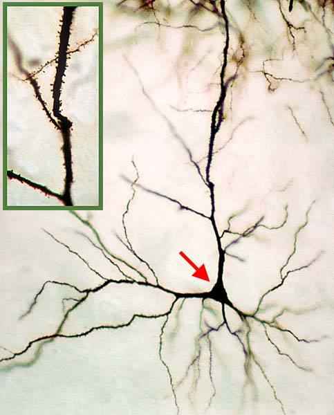
The “pyramidal” part is the cell body, marked with an arrow. The branching lines surrounding the cell body form a tree (or arbor) of dendrites, each of which is covered in tiny dendritic spines (the little barbs visible in the inset picture). Each spine represents a connection, called a synapse, with another neuron from which it can receive signals. A typical cell in the neocortex potentially receives input from several thousand others.

There are two types of dendrite in a pyramidal cell. The first kind, proximal (or near) dendrites, are situated near the cell body and receive almost all their input from “below” in the hierarchy (or from the senses) – this is called feedforward input. The proximal dendrites appear to “add up” the activation signals coming in from below, and will cause the cell to become more and more active depending on the number of incoming signals. When sufficient inputs arrive on the proximal dendrites, the cell may pass a threshold and become active. It will fire off electrical spikes along its axon (or output connection), and this signal will reach all the cells (in this region and others) which receive inputs from the cell. A typical cell might have dozens to a few hundred feedforward connections. Proximal dendrites are responsible for receiving information from the senses (or from other parts of the brain).

The second kind, which accounts for the very large branching seen in the image, are the distal (far) dendrites. These extend quite a distance from the cell body and mainly form connections with nearby cells in the same layer. Distal dendrites are also different in how they respond to their inputs. Unlike the proximal dendrites, which respond in a gradual, linear fashion to a number of inputs across them all, distal dendrites will respond only when a number of signals appear close together along a dendrite segment, and also close together in time. If sufficient coincident inputs are received on a dendrite segment, the cell may become predictive, as if anticipating that it will become active. Distal dendrites are responsible for the information processing within each region.

This is only a tiny subset of all the knowledge we have about the brain, but it’s the core of what we’ll discuss in this book. Let’s move now to the overarching ideas of Jeff Hawkins’ theory – the Memory Prediction Framework.

The Memory Prediction Framework

Jeff Hawkins, the author of the theory, tells the story of how he emerged from Cornell as an engineer, and set out to study the brain and figure out how it worked. He approached the people at the famed MIT Artificial Intelligence Lab, looking for an opportunity to research the brain in order to figure out how it works, and thereby help in the development of computer-based intelligence. He was abruptly told that this was not how it was done, that nobody needed to study how the brain does intelligence in order to build AI programs. The converse happened when he approached the subject in the opposite direction, seeking a research post which would use computational ideas to formulate a working theory of the brain. So, as he relates in his book, On Intelligence, he entered the technology business for a “few years” so that he could fund his own research into a computational theory of the brain.

Fifteen years later, in 2002, having created the PalmPilot and the Handspring Treo, Hawkins set up the Redwood Center for Neurological Research, wrote On Intelligence a year later, and, in 2005, formed Numenta to build a commercial product based on his theory of the brain. This product, Grok, its open-source core, NuPIC, and the underlying theory they’re based on, are the subjects of this book.

The key idea of Hawkins’ initial theory is that the brain is a memory-prediction machine. It receives millions of inputs from the body and eyes - from the world - every second, and uses this information to learn (i.e., create, refine) models of the world which it can then use to make predictions and take actions. This is happening at all scales in the brain, which uses its hierarchy to embody the hierarchical structure of the world (including the structure of our own minds).

In his book, Hawkins outlines his central belief that intelligence is the presence of an internal mechanism which learns, based on sequences of perceptions (patterns), to form a model of the world, uses this to predict future events, and, in turn, may generate new pattern sequences which can often be observed as thought or behaviour. Thought, behaviour, and memory are all equivalent to stored or generated sequences of patterns in the brain. Hawkins’ theory – Hierarchical Temporal Memory – is a model of how the brain literally builds itself out of the never-ending procession of information coming in from the senses.

Let’s look at an example which will illustrate how this works. When you’re listening to someone speaking, your ears receive a very fast stream of sounds which are analysed by an organ called the cochlea in your inner ear. The cochlea, which resembles a snail shell, is an ever-narrowing tube of jelly wound up in a spiral. Embedded in the jelly are tiny hairs which have nerve endings (or receptors) at their bases. As the cochlear tube gets narrower along its length, the passing sound waves will cause the jelly to wobble in sympathy, or resonate, when the width matches the pitch of the sound. This means that each hair, and thus each receptor, will fire in response to a certain pitch (or frequency) range in the sound.

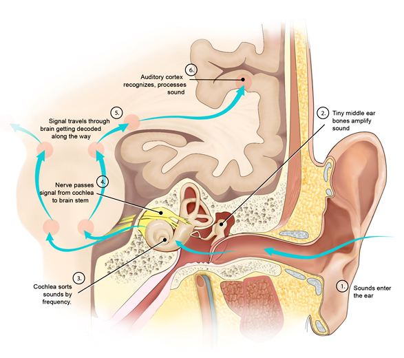
We have about 30,000 separate receptors in our ears, so as you listen to someone talking, your brain is receiving a fast-changing stream of signals along 30,000 separate channels at the same time. Most of these signals will be off, with perhaps only 5-10% of them on. The first region in the cortex to receive this information is the primary auditory cortex (known as A1), which appears to be laid out in the same way as the cochlea itself (high frequencies at one end, low frequencies at the other). This is a pattern we see again and again in the brain – the primary sensory regions have a layout (or topology) which matches that of the sense receptors themselves.

The primary sensory regions, such as A1 (and its visual cousin, V1) are there to find what’s known as primitive spatial features in the sensory information. Each column in the region is connected to its own subset of the inputs, and it will fire or not depending on the number of its inputs which are active (or on). Thus, certain combinations of inputs will cause particular combinations of columns to become active. If you were able to watch the region’s columns from above in real time, you would see a fast-changing sequence of patterns, each of which has only a small percentage of columns active at any one time.

The match-up between the patterns of sound information entering A1 from the cochlea, and the resulting patterns of active columns, is of great interest. This match-up (or mapping) of inputs to activation is something which evolves over your entire life. What each column is doing is actually learning to respond in its own way to the set of inputs it receives at each moment. It is learning to recognise some patterns which arise again and again in the sounds you hear. For each pattern, only some of the inputs will be active, and the column learns by improving its connections to those inputs (on its proximal, or feedforward, dendrites) each time the pattern causes a successful firing. Inputs which are seldom active will be disimproved or neglected.

You can now see that the region has many columns, each of which is being fed a slightly different set of inputs, and each of which is tuning its connections to favour the patterns it most regularly receives (hears, in this case). At any given moment, then, the sound information entering the region causes a varying level of potential activation across the region, with each column displaying a certain amount of response to its input patterns. The columns with the most active inputs will fire first, and when they do this, they send out inhibitory signals to their near neighbours in the region. This acts to lower the neighbouring columns’ activity level even more, causing the best column to stand out in the activation pattern across the region.

The result is what is known in the theory as a Sparse Distributed Representation or SDR, which is a crucial idea for understanding how all this works. Each SDR is itself a spatial pattern, but it represents the features of the raw sound information which caused it. The SDR contains a cleaned-up version of the raw data, because only well-learned features will make it through the analysis. In addition, because of the sparseness caused by inhibition, only the most important feature patterns will survive to be seen in the SDR.

At this stage, the analysed information produced by A1 is sent up the hierarchy to a number of secondary regions. Some of these regions will start identifying features in the sounds which are speech-like in character, while others will be concerned with finding the location of the sound source, its music-like features, and so on. As the information is passed up the hierarchy, it is successively analysed for higher-level feature patterns.

Each region, in addition to learning to recognise and respond to spatial patterns, is also learning to recognise sequences of these patterns. This is another crucial idea in the HTM theory, and we’ll explain it in detail later on. We’ll continue now with an outline in the context of the hearing example.

Let’s move up the hierarchy now to a region which identifies speech-like sounds, or phonemes. This region will be mainly receiving SDR-encoded information, perhaps via a few intermediate regions, originating from the primary A1 region. In addition, it’ll have some connection with the part of the brain which creates and controls all the muscles used in speaking. The reason for this is that we learn to speak by listening to what happens when we make sounds using these muscles, and we keep adjusting the muscles until we learn the right patterns to get the sounds we expect to hear. So the “phoneme” region will itself be tuned to speech-like sounds based on both what it hears and what sounds we’ve learned to make in our own speech. This explains why, for example, native Japanese speakers have trouble distinguishing “l” and “r” sounds, or why English speakers have difficulty with tonal languages like Mandarin.

Each phoneme is actually caused by an intricate sequence of choreographed muscle movements, giving rise to a sequence of particular sound patterns. There are only a few dozen to a few hundred phonemes in each language, and so the sound sequences are easy to learn, and easy to distinguish against background noise. Note that there might be a large number of allowed sound patterns, but it’s the sequences which are key to identifying the phonemes.

So, we see that sequences of sound patterns can be combined to identify phonemes. In the same way (in a higher region), sequences of phonemes can be identified as particular words, sequences of words as phrases, and sequences of phrases as sentences. In this way, the hierarchy learns to hear entire sentences, as sequences of sequences of sequences, even though the sound data coming in was composed of thousands of patterns across 30,000 receptors.

And we can do the opposite. We can construct sentences from phrases we’ve learned, and send them down the hierarchy to generate the words, the phonemes, and the muscle movement sequences need to turn those phonemes into speech. This is the key to understanding how the Hierarchical Temporal Memory works.

The Six Principles of the Neocortex

Here are the six principles which Jeff Hawkins proposes are key to how the neocortex works.

1. On-line learning from streaming data

   Everything we know comes ultimately from the constant stream of information coming in through our senses. At every moment, our brain is taking in this data, and adding to the learning done since before you were born. We do not store a copy of all this information – it’s coming in in huge quantities, we’ve limited capacity, and anyway lots of the individual data is not that important. So, we must do our best to turn it into something useful in real time.

2. Hierarchy of Memory Regions

   The world is complex and ever changing, but it has structure. That structure is hierarchical in nature, and so your brain has a hierarchy which reflects that. The hierarchy serves to compress and abstract both in space and time, and allows us to throw around huge amounts of underlying information about the world very efficiently. It also allows us to find and exploit the connections between different, but related concepts and objects.

3. Sequence Memory

   This is one of the key discoveries of the theory. Everything we experience arrives as a sequence of patterns over time. This is obvious in the case of speech, but it’s true of all sensory input.

   Even our vision is not static, as we might suppose. We are constantly moving our eyes in tiny jumps (called saccades) and gathering little updates from around our field of view. What seems like a static image of the world in front of you is actually made from a memory of many, many sequences of brief glimpses, combined with some older memories from some time ago.

   If I lay an object on the palm of my hand, I have only the barest idea what it is. I know how big it is by noticing the places where I can feel it on my hand, and I can tell its approximate shape and weight by feeling how hard it is at various points. Only when I move the object in my hand do I start to sense the details of its shape, texture, and features. It’s the sequence that contains the real information, since a certain object will create a specific sequence of perceptions when manipulated.

4. Sparse Distributed Representations

   This is the second key discovery of the theory, and in recent years is becoming a widely accepted fact in mainstream neuroscience. SDR’s, to remind you, are representations in which we have only a few percent active columns or cells, all the rest being quiet. SDR’s, when they’re produced as they are in the brain, have a number of extremely powerful and useful properties, which are so important that we’ll devote a whole section to them below.

5. All Regions are Sensory and Motor

   Again, this has only been discovered quite recently. We used to think that the sensory and motor parts of the brain were separate, but it turns out that every region has some kind of motor-related output. We don’t really understand how this works in detail, but it’s important to understand that the brain is learning sensorimotor models of the world – the movement is as important a part of the experiences as the new perception caused by that movement.

   This reflects the fact that all sensory nerves are also “motor” nerves as well – they branch as they enter the brain and go to the classic sensory regions in the neocortex, in addition going to motor-related regions in the lower parts of the brain. The signals coming in convey one piece of information, but its meaning can be interpreted as both an item of sensory data (my leg is moving this way) and as an instruction for a corresponding movement to make in the near-future.

6. Attention

   We have the ability to focus our awareness on certain bits of the hierarchy, ignoring much of what is happening elsewhere. If you look at the word “attention” above, you will notice that the rest of the page seems to fade out as you dwell on the word. Now, look at the letter “i” in that word, and you see that you are “zooming in” on that letter. Finally, you can just concentrate on the dot above the i, and you see that your attention can become almost microscopic. If you come across the word attention in a sentence, however, it’ll remain in focus for only a fraction of a second.

Realising the Theory: The Cortical Learning Algorithm

These six principles are, Hawkins claims, both necessary and sufficient for intelligence. In order to establish this, however, we’ll need to go beyond declaring the principles and create a detailed theoretical model of how these principles actually work, and then we can build computer systems based on these details.

In 2009, Hawkins and his team at Numenta made some significant breakthroughs in their work on HTM, which led to a new “sub-theory” called the Cortical Learning Algorithm (CLA). The CLA is a realisation in detail of these three central principles of HTM:

• On-line learning from streaming data
• Sequence Memory
• Sparse Distributed Representations

We’ll go into some detail on the CLA in the next Chapter.

In 2013 and early 2014, Hawkins has expanded the CLA to model two more of the six Principles:

• Hierarchy of Memory Regions
• All Regions are Sensory and Motor

This new theory, which I call Sensorimotor CLA, is a huge expansion and is still the subject of animated discussion on the community’s theory mailing list, so please treat my descriptions as preliminary and subject to revision.