Three: The Cortical Learning Algorithm
The Cortical Learning Algorithm is a detailed mechanism for explaining the operation of a single-layer, single region of neocortex. This region is capable of learning sequences of spatial-temporal data, making predictions, and detecting anomalies in the data.
NuPIC and its commercial version, Grok, are realisations in software of the CLA, allowing us to observe how the model performs and also put it to work solving real-world problems.
The CLA Model Neuron
As described above, we know a lot about how individual neurons work in the neocortex. While each of the tens of billions of neurons in each of our brains is unique and very complex, for our purposes they can each be replaced with a standard neuron which looks like this:
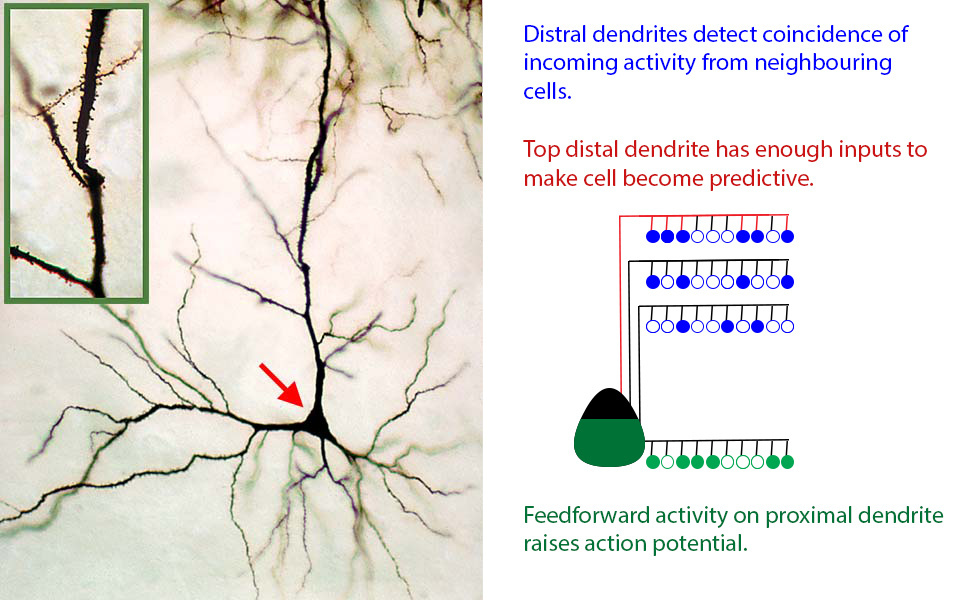
Real (left) and CLA model (right) neurons
This model neuron is a significant simplification, but it captures the most important characteristics of real neurons. The key features are:
- The neuron receives feedforward inputs at the proximal dendrites (bottom, green), each active input raising the action potential of the cell (green filling of the cell body).
- If enough active signals come in at the proximal dendrites, the cell may become active and begin firing off its own signal.
- Signals from other neurons (mostly nearby, mostly in the same region) are connected at a particular piece, or segment of the distal dendrite arbor (top, blue).
- If enough signals appear on a segment, the segment (red, top segment) will cause the cell to become predictive of its own activity (red line).
This model neuron, while dramatically less complex and variable than a real one, is nevertheless a lot more complicated than the neurons found in other neural network systems.
When it comes to modelling the signals, we also use a simplified model of the real thing. The incoming signal is modelled by a “bit” - active or inactive, 1 or 0 - instead of the more realistic scalar value which would represent the signalling neuron’s firing rate or voltage.
The synapse (the junction between a signalling neuron and the receiving dendrite) is simplified too. It has a permanence which models the growth (or shrinkage) of the dendritic spine reaching out to the incoming neuron’s axon - this varies from 0.0 to 1.0. Secondly, the synapse is either “connected” or not - again a 1 or 0, based on whether the permanence is above or below a threshold. We will later see that this permanence is the key to learning - raising the permanence over time allows the CLA to “remember” a useful connection, while lowering it (due to disuse) allows it to “forget” that connection.
The CLA Model of a Neocortical Region
As we noted earlier, the neocortex is divided up into patches or regions of various sizes. A region is identified by the source of its feedforward inputs; for example, the primary auditory cortex A1 is identified as the receiver of the sound information coming in from the cochlea.
Each region in the real neocortex has five or six layers of neurons connected together in a very complex manner. The layered structure allows the region to perform some very complex processing, which combines information coming in from lower regions (or the senses), higher regions (feedback, “instructions” and attention control), and the information stored in the region itself (spatial-temporal memory).
At this stage in the development of the theory, we create a very simplified region which could be seen as a model of a single layer in the real neocortex. This consists of a two-dimensional grid of columns, each of which is a stack of our model neurons.
Before proceeding any further, we should take a look at a really important concept in HTM: Sparse Distributed Representations.
Sparse Distributed Representations
SDR’s are the currency of intelligence, both in the brain and in machine intelligence. Only SDR’s have the unique characteristics which allow us to learn, build and use robust models of the world based on experience and thought. This section explains why this way of representing a perception or an idea is so important.
SDR’s are sparse: in each example, there are many possible neurons, columns, or bits which could be on; however, most of them are inactive, quiet, or off. In NuPIC, for example, 2% of columns are used (typically, 40 out of 2,000 columns are active at any time). This may seem like a waste of neurons, but as we’ll see, there are some serious benefits to this.
SDR’s are distributed: the active cells are spread out across the region in an apparently random pattern. Over time, the patterns will visit all parts of the region and all cells will be involved in representing the activity of the region (if only for a small proportion of the time).
In addition, and very importantly, each active cell in an SDR has semantic meaning of some sort which comes from the structure in the inputs which caused it to become active. Each cell may be thought of as capturing some “feature” in the inputs, an example from vision being a vertical line in a certain place. But because the SDR is distributed, it’s important to note that no single cell is solely responsible for representing each feature - that responsibility is shared among a number of other active cells in each SDR.
Important Properties of SDRs
SDRs have some very important properties which, when combined, may prove crucial to their use both in the brain and in machine intelligence.
Efficiency by Indexing
In software, we can clearly store large SDRs very efficiently by just storing the locations of the active, or 1-bits, instead of storing all the zeros as well. In addition, we can compare two SDRs very quickly simply by comparing their active bits.
In the brain, the sparsity of neuronal activity allows for efficient use of energy and resources, by ensuring that only the strongest combinations of meaningful signals lead to activation, and that memory is used to store information of value.
Subsampling and Semantic Overlap
Because every active bit or neuron signifies some significant semantic information in the input, the mathematics of SDRs means that a subsampled SDR is almost as good as the whole representation. This means that any higher-level system which is “reading” the SDR needs only a subset of bits to convey the representation. In turn, this feature leads to greater fault-tolerance and robustness in the overall system.
The math also indicates that when two SDRs differ by a few bits, we can be highly confident that they are representing the same underlying thing, and even if this is not the case, the error is between two very semantically similar inputs.
Unions of SDRs
SDRs, like any bitmaps, can be combined in many ways. The most important combination in HTM is the (inclusive) OR operation, which turns on a bit if either or both inputs have that bit on. When the bitmaps are sparse, the OR (or union) will mostly contain bits from one or other of the inputs, with just a few bits shared commonly between them.
Given a set of SDRs (each representing one sensory experience, for example), the union will in a way represent the possibility of all members of the set. The union process is irreversible: all the bits are mixed together, so we cannot recover individual members. However, we can say with high confidence that a newly presented SDR is a member of the union.
This is very important for HTM, because it underlies the prediction process. When an HTM layer is making a prediction, it does so by combining all its predictions in a union of SDRs, and we can check if something is predicted by asking if its SDR is contained in this union.
Creating a Sparse Distributed Representation: Pattern Memory (Spatial Pooling)
Now that we have a basic understanding of SDRs, let’s look at how the CLA uses the structure of a layer to represent a sensory input as an SDR. This process has been called Spatial Pooling, because the layer is provided with a spatial pattern of active bits, and it is pooling the information from all these bits and forming a single SDR which (it is hoped) signifies the structure in the sensory data.
Later, we will see that this process is used for more complex things than spatial sensory patterns, so we’ll drop “Spatial Pooling” in favour of “Pattern Memory” in later discussions. For now, these are equivalent.
To make it simple for now, imagine that the neurons in each column are so similar that we can pretend each column contains only a single cell. We will add back the complexity later when we introduce sequence memory.
The layer now looks like a 2-dimensional grid (i.e., array) of single cells. Each cell has a proximal, or feedforward dendrite, which receives some input from the senses or a lower region in the hierarchy. Not every input bit is connected to every cell, so each cell will receive a subset of the input signal (we say it subsamples the input). We’ll assume that each cell receives a unique selection of subsampled bits. In addition, at any given moment, the synapses on a cell’s dendrites will each have some permanence, and this will further control how input signals are transmitted into the cell.
When an input appears, each active bit in the input signal will be transmitted only to a subset of cell dendrites in the layer (those which have that bit in their subsample or potential pool), and these signals will then continue only where the synapse permanence is sufficient to allow them through. Each cell thus acts as a kind of filter, receiving inputs from quite a small subsample of the incoming signal. If many bits from this subsample happen to be active, the cell will “charge up” with a high activation potential; on the other hand, if a cell has mostly off-bits in its receptive field, or if many of the synapses have low permanence, the total effect on the cell will be minimal, and its activation potential will be small or zero.
At this stage, we can visualise the layer as forming a field of activation potentials, with each cell in the grid possessing a level of activation potential (in the real brain, the cell membranes each have a real voltage, or potential). We now need to turn this into a binary SDR, and we do this using a strategy called “winner-takes-all” in machine learning, or “inhibition” in neuroscience and HTM.
The essential idea is to choose the cells with the highest potential to make active, and allow the lower potential cells be inhibited or suppressed by the winners. In HTM, we can do this either “globally”, by picking the highest n% potentials in a whole layer, or “locally”, by splitting the layer into neighbourhoods and choosing one or a few cells from each. The best choice depends on whether we wish to model the spatial structure of SDRs directly in the layout of the active cells - as happens in primary visual cortex V1, for example.
In the neocortex, each column of cells has a physical “sheath” of inhibitory cells, which are triggered if the column becomes active. These cells are very fast-acting, so they will almost instantly suppress the adjacent columns’ activity once triggered by a successful firing. In addition, these inhibitory cells are connected to each other, so a wave of inhibition will quickly spread out from an active column, leaving it isolated in an area of inactivity. This simple mechanism is sufficient to enforce almost all of the sparseness we see in the neocortex (there are many other mechanisms in the real cortex, but this is good enough for now).
The result is an SDR of active columns, which is the result of Spatial Pooling.
If this looks just like pattern recognition to you, you’d be correct. And you’d also be correct if you guessed how this process involves reinforcement learning, because this idea is common across many types of artificial neural networks. In most of these, there are numeric weights instead of our synapses, and these weights are adjusted so as to strengthen the best-matching connections between inputs and neurons. In the CLA, we instead adjust the permanence of the synapses. If the cell becomes active, we increase the permanence of any synapses which are attached to on-bits in the input, and we decrease slightly the permanence of synapses connected to the off-bits.
In this way (the mathematical properties of this kind of learning are discussed in detail elsewhere), each cell will gradually become better and better at recognising the subset of the inputs it sees most commonly over time, and so it’ll become more likely to become active when these, or similar, inputs appear again.
Prediction Part I - Transition Memory
The key to the power of CLA is in the combination of Pattern Memory with the ability to learn, “understand,” and predict how the patterns in the world change over time, and how these changes have a sequence-like structure which reflects structure in the real world. We now believe that all our models of reality (including our own internal world) are formed from memories of this nature.
We’ll now extend the theory a little to show how the CLA learns about individual steps in the changing sensory stream it experiences, and how these changes are chained together to form sequence memories. Again, we’ll need to postpone the full details in favour of a deep understanding of just this phase in the process.
Active Columns to Active Cells
Picking up the discussion from the last section on Pattern Memory (Spatial Pooling), remember that we pretended each column had only one cell when looking at the spatial patterns coming in from the senses. This was good enough to give us a way to recognise recurring structure in each pattern we saw, and form a “pooled” SDR on the layer which represented that pattern.
We now want to look at what happens when these patterns change (as all sensory input continually does), and how the CLA learns the structural information in these changes - we call them transitions - attempts to predict them and spot if something unexpected happens. We call this process Transition Memory (some people - including Jeff - call this Temporal Memory, but I like my term better!).
Pattern Memory in the last section used only the feedforward, or proximal, dendrites of each cell to look at the sensory inputs as they appeared. In learning transitions and making predictions, we use the remaining, distal dendrites to learn how one pattern leads onto the next. This is the key to the power of CLA in learning the spatiotemporal structure of the world.
In order to make this work, we must put back all the cells in each column, because it’s the way the cells behave which allows the transitions to be learned and predictions to be made. So, in each active column, we now have several dozen cells (in NuPIC we usually use 32) and we have to decide what is happening at this level of detail.
We’ll assume for now (and explain later) that in each active column, only one of the cells is active and the others are quiescent. Each active cell is sending out a signal on its axon (this is the definition of being active), and this axon has a branching structure a bit like the structure of the dendrites. Many axonal branches spread out horizontally in the layer and connect up with the dendrites of cells in neighbouring columns (perhaps spreading across distances many columns wide).
We’ll thus see (and can record) a spreading signal which connects currently active cells in some columns to many thousands of cells in many other columns. Some of the cells receiving these signals will happen to be connected to significant numbers of active cells, and some of these will happen to receive several signals close together on the same segment of a dendrite. If this happens, the segment will generate a dendritic spike (which is quite similar to the spike generated by an axon when it fires), and this spike will travel down the dendrite until it reaches the cell body. Each dendritic spike injects some small amount of electrical current into the cell body, and this raises the voltage across its membrane - a process called depolarisation.
Of course, many cells in the layer will receive little or no signals from the small number of active cells, and even if they do, the signals might appear on different branches and at different times. These signals will not appear close together enough to exceed a dendrite segment’s spiking threshold, and they will effectively be ignored. This means that, over the layer, we would be able to observe a second sparse pattern (or field) - this time of depolarisation caused by the signals between cells in the layer. Most cells will have zero depolarisation (they’ll be at a “resting potential”), but some cells will have a little and some will be highly depolarised.
This new pattern of depolarisation in the layer is a result of cells combining signals from the recently active pattern of cells we saw generated in the Pattern Memory phase. The key to the whole Transition Memory process is that this second pattern is used to combine this signal from the recent past with the next sensory pattern which appears a short time later. Cells which are depolarised strongly by both the distal dendritic spikes (from cells in the recent past), and by the incoming, new sensory signal will have a head-start in reaching their firing threshold and will be the best bet to be among the top few percent picked to be in the next spatial pooling SDR.
We call cells which possess a high level of depolarisation due to horizontal signals predictive, since they will use this depolarisation to predict their own activity - if and when their expected sensory pattern arrives. If the prediction is correct, these cells will indeed become active, and they’ll do the same kind of reinforcement learning we saw in the previous section. Thus the layer learns how to associate the previous pattern with likely patterns coming next. This is the kernel of Transition Memory.
Prediction Part II - Sequence Memory
We saw in the previous section that a layer of cells arranged in columns can learn to predict individual transitions from one feedforward pattern to another. This Transition Memory has another key feature - the ability to learn high-order sequences of patterns, which turns out to be the key to intelligence. Let’s see how this works.