Leanpub: Publish Early, Publish Often

Appendix 4: Mathematics of HTM

This article describes some of the mathematics underlying the theory and implementations of Jeff Hawkins’ Hierarchical Temporal Memory (HTM), which seeks to explain how the neocortex processes information and forms models of the world.

The HTM Model Neuron - Pattern Memory (aka Spatial Pooling)

We’ll illustrate the mathematics of HTM by describing the simplest operation in HTM’s Cortical Learning Algorithm: Pattern Memory, also known as Spatial Pooling, forms a Sparse Distributed Representation from a binary input vector. We begin with a layer (a 1- or 2-dimensional array) of single neurons, which will form a pattern of activity aimed at efficiently representing the input vectors.

Feedforward Processing on Proximal Dendrites

The HTM model neuron has a single proximal dendrite, which is used to process and recognise feedforward or afferent inputs to the neuron. We model the entire feedforward input to a cortical layer as a bit vector ${\mathbf x}_ {\textrm{ff}}\in\lbrace{0,1}\rbrace^ {n_ {\textrm{ff}}}$ , where $n_ {\textrm{ff}}$ is the width of the input.

The dendrite is composed of n_ s synapses which each act as a binary gate for a single bit in the input vector. Each synapse has a permanence $p_ i\in{[0,1]}$ which represents the size and efficiency of the dendritic spine and synaptic junction. The synapse will transmit a 1-bit (or on-bit) if the permanence exceeds a threshold $\theta_ i$ (often a global constant $\theta_ i = \theta = 0.2$ ). When this is true, we say the synapse is connected.

Each neuron samples n_ s bits from the $n_ {\textrm{ff}}$ feedforward inputs, and so there are ${n_ {\textrm{ff}}}\choose{n_ {s}}$ possible choices of input for a single neuron. A single proximal dendrite represents a projection $\pi_ j:\lbrace{0,1}\rbrace^ {n_ {\textrm{ff}}}\rightarrow\lbrace{0,1}\rbrace^ {n_ s}$ , so a population of neurons corresponds to a set of subspaces of the sensory space. Each dendrite has an input vector ${\mathbf x}_ j=\pi_ j({\mathbf x}_ {\textrm{ff}})$ which is the projection of the entire input into this neuron’s subspace.

A synapse is connected if its permanence p_ i exceeds its threshold $\theta_ i$ . If we subtract ${\mathbf p}-{\vec\theta}$ , take the elementwise sign of the result, and map to $\lbrace{0,1}\rbrace$ , we derive the binary connection vector ${\mathbf c}_ j$ for the dendrite. Thus:

$c_ i=(1 + sgn(p_ i-\theta_ i))/2$

The dot product $o_ j({\mathbf x})={\mathbf c}_ j\cdot{\mathbf x}_ j$ now represents the feedforward overlap of the neuron with the input, ie the number of connected synapses which have an incoming activation potential. Later, we’ll see how this number is used in the neuron’s processing.

The elementwise product ${\mathbf o}_ j={\mathbf c}_ j\odot{\mathbf x}_ j$ is the vector in the neuron’s subspace which represents the input vector ${\mathbf x}_ {\textrm{ff}}$ as “seen” by this neuron. This is known as the overlap vector. The length $o_ j = \lVert{\mathbf o}_ j\rVert_ {\ell_ 1}$ of this vector corresponds to the extent to which the neuron recognises the input, and the direction (in the neuron’s subspace) is that vector which has on-bits shared by both the connection vector and the input.

If we project this vector back into the input space, the result $\mathbf{\hat{x}}_ j =\pi^ {-1}({\mathbf o}_ j)$ is this neuron’s approximation of the part of the input vector which this neuron matches. If we add a set of such vectors, we will form an increasingly close approximation to the original input vector as we choose more and more neurons to collectively represent it.

Sparse Distributed Representations (SDRs)

We now show how a layer of neurons transforms an input vector into a sparse representation. From the above description, every neuron is producing an estimate $\mathbf{\hat{x}}_ j$ of the input ${\mathbf x}_ {\textrm{ff}}$ , with length $o_ j\ll n_ {\textrm{ff}}$ reflecting how well the neuron represents or recognises the input. We form a sparse representation of the input by choosing a set $Y_ {\textrm{SDR}}$ of the top $n_ {\textrm{SDR}}=sN$ neurons, where is the number of neurons in the layer, and is the chosen sparsity we wish to impose (typically $s=0.02=2\%$ ).

The algorithm for choosing the top $n_ {\textrm{SDR}}$ neurons may vary. In neocortex, this is achieved using a mechanism involving cascading inhibition: a cell firing quickly (because it depolarises quickly due to its input) activates nearby inhibitory cells, which shut down neighbouring excitatory cells, and also trigger further nearby inhibitory cells, spreading the inhibition outwards. This type of local inhibition can also be used in software simulations, but it is expensive and is only used where the design involves spatial topology (ie where the semantics of the data is to be reflected in the position of the neurons). A more efficient global inhibition algorithm - simply choosing the top $n_ {\textrm{SDR}}$ neurons by their depolarisation values - is often used in practise.

If we form a bit vector ${\mathbf y}_ {\textrm{SDR}}\in\lbrace{0,1}\rbrace^ N\textrm{ where } y_ j = 1 \Leftrightarrow j \in Y_ {\textrm{SDR}}$ , we have a function which maps an input ${\mathbf x}_ {\textrm{ff}}\in\lbrace{0,1}\rbrace^ {n_ {\textrm{ff}}}$ to a sparse output ${\mathbf y}_ {\textrm{SDR}}\in\lbrace{0,1}\rbrace^ N$ , where the length of each output vector is $\lVert{\mathbf y}_ {\textrm{SDR}}\rVert_ {\ell_ 1}=sN \ll N$ .

The reverse mapping or estimate of the input vector by the set $Y_ {\textrm{SDR}}$ of neurons in the SDR is given by the sum:

$\mathbf{\hat{x}} = \sum\limits_ {j \in Y_ {\textrm{SDR}}}{{\mathbf{\hat{x}}}_ j} = \sum\limits_ {j \in Y_ {\textrm{SDR}}}{\pi_ j^ {-1}({\mathbf o}_ j)} = \sum\limits_ {j \in Y_ {\textrm{SDR}}}{\pi_ j^ {-1}({\mathbf c}_ j\odot{\mathbf x}_ j)}= \sum\limits_ {j \in Y_ {\textrm{SDR}}}{\pi_ j^ {-1}({\mathbf c}_ j \odot \pi_ j({\mathbf x}_ {\textrm{ff}}))}= \sum\limits_ {j \in Y_ {\textrm{SDR}}}{\pi_ j^ {-1}({\mathbf c}_ j) \odot {\mathbf x}_ {\textrm{ff}}}$

Matrix Form

The above can be represented straightforwardly in matrix form. The projection $\pi_ j:\lbrace{0,1}\rbrace^ {n_ {\textrm{ff}}} \rightarrow\lbrace{0,1}\rbrace^ {n_ s}$ can be represented as a matrix $\Pi_ j \in \lbrace{0,1}\rbrace^ {{n_ s} \times\ n_ {\textrm{ff}}}$ .

Alternatively, we can stay in the input space $\mathbb{B}^ {n_ {\textrm{ff}}}$ , and model $\pi_ j$ as a vector $\vec\pi_ j =\pi_ j^ {-1}(\mathbf 1_ {n_ s})$ , ie where $\pi_ {j,i} = 1 \Leftrightarrow (\pi_ j^ {-1}(\mathbf 1_ {n_ s}))_ i = 1$ .

The elementwise product $\vec{x_ j} =\pi_ j^ {-1}(\mathbf x_ {j}) = \vec{\pi_ j} \odot {\mathbf x_ {\textrm{ff}}}$ represents the neuron’s view of the input vector $x_ {\textrm{ff}}$ .

We can similarly project the connection vector for the dendrite by elementwise multiplication: 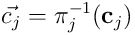$\vec{c_ j} =\pi_ j^ {-1}(\mathbf c_ {j})$ , and thus 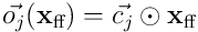$\vec{o_ j}(\mathbf x_ {\textrm{ff}}) = \vec{c_ j} \odot \mathbf{x}_ {\textrm{ff}}$ is the overlap vector projected back into $\mathbb{B}^ {n_ {\textrm{ff}}}$ , and the dot product 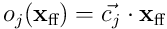$o_ j(\mathbf x_ {\textrm{ff}}) = \vec{c_ j} \cdot \mathbf{x}_ {\textrm{ff}}$ gives the same overlap score for the neuron given $\mathbf x_ {\textrm{ff}}$ as input. Note that 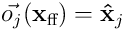$\vec{o_ j}(\mathbf x_ {\textrm{ff}}) =\mathbf{\hat{x}}_ j$ , the partial estimate of the input produced by neuron .

We can reconstruct the estimate of the input by an SDR of neurons $Y_ {\textrm{SDR}}$ :

$\mathbf{\hat{x}}_ {\textrm{SDR}} = \sum\limits_ {j \in Y_ {\textrm{SDR}}}{{\mathbf{\hat{x}}}_ j} = \sum\limits_ {j \in Y_ {\textrm{SDR}}}{\vec o}_ j = \sum\limits_ {j \in Y_ {\textrm{SDR}}}{{\vec c}_ j\odot{\mathbf x_ {\textrm{ff}}}} = {\mathbf C}_ {\textrm{SDR}}{\mathbf x_ {\textrm{ff}}}$

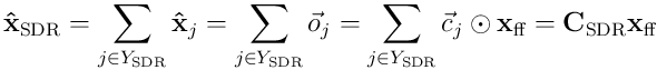
where ${\mathbf C}_ {\textrm{SDR}}$ is a matrix formed from the ${\vec c}_ j$ for $j \in Y_ {\textrm{SDR}}$ .

Optimisation Problem

We can now measure the distance between the input vector $\mathbf x_ {\textrm{ff}}$ and the reconstructed estimate $\mathbf{\hat{x}}_ {\textrm{SDR}}$ by taking a norm of the difference. Using this, we can frame learning in HTM as an optimisation problem. We wish to minimise the estimation error over all inputs to the layer. Given a set of (usually random) projection vectors $\vec\pi_ j$ for the N neurons, the parameters of the model are the permanence vectors $\vec{p}_ j$ , which we adjust using a simple Hebbian update model.

The update model for the permanence of a synapse p_ i on neuron is:

$p_ i^ {(t+1)} = \begin{cases} (1+\delta_ {inc})p_ i^ {(t)} & \text{if } j \in Y_ {\textrm{SDR}}\text{, }(\mathbf x_ j)_ i=1\text{ and } p_ i^ {(t)} \ge \theta_ i \\ (1-\delta_ {dec})p_ i^ {(t)} & \text{if } j \in Y_ {\textrm{SDR}} \text{ and (}(\mathbf x_ j)_ i=0 \text{ or }p_ i^ {(t)} < \theta_ i \text{)} \\ p_ i^ {(t)} & \text{otherwise} \\ \end{cases}$

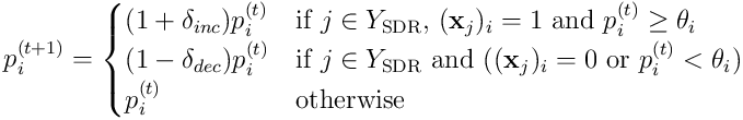
This update rule increases the permanence of active synapses, those that were connected to an active input when the cell became active, and decreases those which were either disconnected or received a zero when the cell fired. In addition to this rule, an external process gently boosts synapses on cells which either have a lower than target rate of activation, or a lower than target average overlap score.

I do not yet have the proof that this optimisation problem converges, or whether it can be represented as a convex optimisation problem. I am confident such a proof can be easily found. Perhaps a kind reader who is more familiar with a problem framed like this would be able to confirm this. I’ll update this post with more functions from HTM in coming weeks.

Transition Memory - Making Predictions

In Part One, we saw how a layer of neurons learns to form a Sparse Distributed Representation (SDR) of an input pattern. In this section, we’ll describe the process of learning temporal sequences.

We showed in part one that the HTM model neuron learns to recognise subpatterns of feedforward input on its proximal dendrites. This is somewhat similar to the manner by which a Restricted Boltzmann Machine can learn to represent its input in an unsupervised learning process. One distinguishing feature of HTM is that the evolution of the world over time is a critical aspect of what, and how, the system learns. The premise for this is that objects and processes in the world persist over time, and may only display a portion of their structure at any given moment. By learning to model this evolving revelation of structure, the neocortex can more efficiently recognise and remember objects and concepts in the world.

Distal Dendrites and Prediction

In addition to its one proximal dendrite, a HTM model neuron has a collection of distal (far) dendrite segments (or simply dendrites), which gather information from sources other than the feedforward inputs to the layer. In some layers of neocortex, these dendrites combine signals from neurons in the same layer as well as from other layers in the same region, and even receive indirect inputs from neurons in higher regions of cortex. We will describe the structure and function of each of these.

The simplest case involves distal dendrites which gather signals from neurons within the same layer.

In Part One, we showed that a layer of neurons converted an input vector $\mathbf x \in \mathbb{B}^ {n_ {\textrm{ff}}}$ into a SDR $\mathbf{y}_ {\textrm{SDR}} \in \mathbb{B}^ {N}$ , with length $\lVert{\mathbf y}_ {\textrm{SDR}}\rVert_ {\ell_ 1}=sN \ll N$ , where the sparsity is usually of the order of 2% ( is typically 2048, so the SDR $\mathbf{y}_ {\textrm{SDR}}$ will have 40 active neurons).

The layer of HTM neurons can now be extended to treat its own activation pattern as a separate and complementary input for the next timestep. This is done using a collection of distal dendrite segments, which each receive as input the signals from other neurons in the layer itself. Unlike the proximal dendrite, which transmits signals directly to the neuron, each distal dendrite acts individually as an active coincidence detector, firing only when it receives enough signals to exceed its individual threshold.

We proceed with the analysis in a manner analogous to the earlier discussion. The input to the distal dendrite segment at time is a sample of the bit vector $\mathbf{y}_ {\textrm{SDR}}^ {(t-1)}$ . We have $n_ {ds}$ distal synapses per segment, a permanence vector $\mathbf{p}_ k \in [0,1]^ {n_ {ds}}$ and a synapse threshold vector $\vec{\theta}_ k \in [0,1]^ {n_ {ds}}$ , where typically $\theta_ i = \theta = 0.2$ for all synapses.

Following the process for proximal dendrites, we get the distal segment’s connection vector $\mathbf{c}_ k$ :

$c_ {k,i}=(1 + sgn(p_ {k,i}-\theta_ {k,i}))/2$

The input for segment is the vector 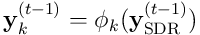$\mathbf{y}_ k^ {(t-1)} = \phi_ k(\mathbf{y}_ {\textrm{SDR}}^ {(t-1)})$ formed by the projection 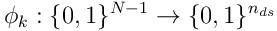$\phi_ k:\lbrace{0,1}\rbrace^ {N-1}\rightarrow\lbrace{0,1}\rbrace^ {n_ {ds}}$ from the SDR to the subspace of the segment. There are ${N-1}\choose{n_ {ds}}$ such projections (there are no connections from a neuron to itself, so there are N-1 to choose from).

The overlap of the segment for a given $\mathbf{y}_ {\textrm{SDR}}^ {(t-1)}$ is the dot product 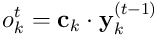$o_ k^ t = \mathbf{c}_ k\cdot\mathbf{y}_ k^ {(t-1)}$ . If this overlap exceeds the threshold $\lambda_ k$ of the segment, the segment is active and sends a dendritic spike of size s_ k to the neuron’s cell body.

This process takes place before the processing of the feedforward input, which allows the layer to combine contextual knowledge of recent activity with recognition of the incoming feedforward signals. In order to facilitate this, we will change the algorithm for Pattern Memory as follows.

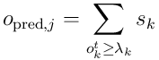
Each neuron begins a timestep by performing the above processing on its ${n_ {\textrm{dd}}}$ distal dendrites. This results in some number $0\ldots{n_ {\textrm{dd}}}$ of segments becoming active and sending spikes to the neuron. The total predictive activation potential is given by:

$o_ {\textrm{pred},j}=\sum\limits_ {o_ k^ {t} \ge \lambda_ k}{s_ k}$

The predictive potential is combined with the overlap score from the feedforward overlap coming from the proximal dendrite to give the total activation potential:

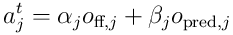
$a_ j^ t=\alpha_ j o_ {\textrm{ff},j} + \beta_ j o_ {\textrm{pred},j}$

and these a_ j potentials are used to choose the top neurons, forming the SDR $Y_ {\textrm{SDR}}$ at time . The mixing factors $\alpha_ k$ and $\beta_ k$ are design parameters of the simulation.

Learning Predictions

We use a very similar learning rule for distal dendrite segments as we did for the feedforward inputs:

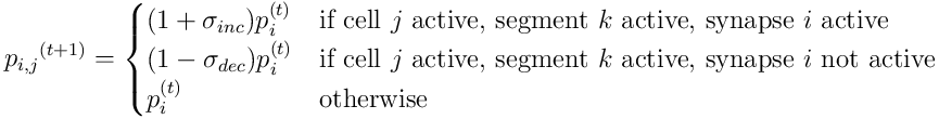
${p_ {i,j}}^ {(t+1)} = \begin{cases} (1+\sigma_ {inc})p_ i^ {(t)} & \text {if cell } j \text{ active, segment } k \text{ active, synapse } i \text{ active} \\ (1-\sigma_ {dec})p_ i^ {(t)} & \text {if cell } j \text { active, segment } k \text{ active, synapse } i \text{ not active} \\ p_ i^ {(t)} & \text{otherwise} \\ \end{cases}$

Again, this reinforces synapses which contribute to activity of the cell, and decreases the contribution of synapses which don’t. A boosting rule, similar to that for proximal synapses, allows poorly performing distal connections to improve until they are good enough to use the main rule.

Interpretation

We can now view the layer of neurons as forming a number of representations at each timestep. The field of predictive potentials $o_ {\textrm{pred},j}$ can be viewed as a map of the layer’s confidence in its prediction of the next input. The field of feedforward potentials $o_ {\textrm{ff},j}$ can be viewed as a map of the layer’s recognition of current reality. Combined, these maps allow for prediction-assisted recognition, which, in the presence of temporal correlations between sensory inputs, will improve the recognition and representation significantly.

We can quantify the properties of the predictions formed by such a layer in terms of the mutual information between the SDRs at time and t+1 . I intend to provide this analysis as soon as possible, and I’d appreciate the kind reader’s assistance if she could point me to papers which might be of help.

A layer of neurons connected as described here is a Transition Memory, and is a kind of first-order memory of temporally correlated transitions between sensory patterns. This kind of memory may only learn one-step transitions, because the SDR is formed only by combining potentials one timestep in the past with current inputs.

Since the neocortex clearly learns to identify and model much longer sequences, we need to modify our layer significantly in order to construct a system which can learn high-order sequences. This is the subject of the next part of this Appendix.

Note: For brevity, I’ve omitted the matrix treatment of the above. See Part One for how this is done for Pattern Memory; the extension to Transition Memory is simple but somewhat arduous.