7 Data logging and handling
We already mentioned several times how to log your data in NeuroTask Scripting. The basic function for this is log(), which adds a row of new data to the data table in your account. For most experiments this type of storage is sufficient In other words, data logging is easy and the form controls such as input(), check(), and scale() log the subject’s responses automatically. This chapter describes the rest of the data management system, including a few cases where you need more options to store and perhaps retrieve data.
As an example of why you would want to store and retrieve some data, consider the case that you invite a certain group of patients to take a test battery that consists of three fairly long tests (say 12 min each). Some patients may get interrupted and then later return to the test battery. In such a case, it would be handy if you could somehow retrieve which parts of the test battery that had already taken, so that you could skip these when they return. For these and several other use cases, NeuroTask Scripting has functions that let you not only log but also update and retrieve data in a running script.
In this chapter, we will first discuss the log() function. Then, we will tell a few things about where your data ends up, some tricks to get a better view on your data, and how to download it. Finally, we will discuss how you could store and retrieve data for more complicated situations.
7.1 Data logging with log()
The log() function is the basis of all data logging. NeuroTask Scripting distinguishes between data logging and storing: Data logging never overwrites existing data and always adds a new row to your data table. Data storing, however, will overwrite the data row in your table if it has the same label. We will discuss data storing towards the end of this chapter.
To log some data, you can simply write:
log(42,"var3");
This will add a row of data to the data table in your account with name ‘var3’. It will also include a timestamp with the exact date and time when the data was logged. And it will have information about the subject and session.
In most cases, you will first collect a response from a participant in a variable and then log its value:
 1 var e, b;
 2
 3 b = addblock().text("Get ready to click with the (left) mouse button...");
 4 await(4000);
 5 b.clear();
 6
 7 await(randint(1000,3000);
 8 b.text("Now");
 9 e = b.await("click");
10
11 log(e.RT,"Reaction Time");
12 await(5000);
This script is a simple reaction time task. First, a text appears on the screen with the text ‘Get ready to click with the (left) mouse button…’. After 4 s the text disappears and after a random interval of 1 to 3 s the text ‘Now’ appears. We use the randint(min,max) function which generates a random integer in the range min to (but not including) max. The click event is caught by the await() function its return value capture in variable e. As explained in the chapter on events, the return value already contains a property RT that holds the reaction time, which we log as shown.
For reaction times, we would normally like to run several trials and then average these. This can be done with a for loop. Let’s run ten trials and adjust the script accordingly:
 1 var e, b, i;
 2
 3 b = addblock();
 4
 5 for (i = 0; i < 10; ++i)
 6 {
 7     b.text("Get ready to click with the (left) mouse button...");
 8     await(2000);
 9     b.clear();
10
11     await(randint(1000,3000);
12     b.text("Now");
13     e = b.await("click");
14
15     log(e.RT,"Reaction Time");
16     await(1500);
17 }
18
19 await(5000);
This script has a for loop that runs ten times. We have moved creating of the block outside the loop, because we don’t want to create it ten times; we just want to show the instruction text ten times. We have also add a 1.5 s wait at the end of the loop so that after clicking the participant gets a brief pause. We shortened the time the instruction is shown to 2 s, because 4 s felt quite long if you run several trials.
Script 7.2 will log ‘Reaction Time’ ten times, each time with different values, which will show up as rows in your data table. Once you have downloaded the table (discussed below) you could analyze the reaction times, for example, in Excel. To facilitate this and to give the participant some feedback, let’s keep track of the total time in a variable named total, calculate the average reaction time and assign to variable average, log this variable, and use it to give some feedback to the participant.
 1 var e, b, i, total, average;
 2
 3 total = 0;
 4
 5 b = addblock();
 6
 7 for (i = 0; i < 10; ++i)
 8 {
 9     b.text("Get ready to click with the (left) mouse button...");
10     await(2000);
11     b.clear();
12
13     await(randint(1000,3000);
14     b.text("Now");
15     e = b.await("click");
16
17     log(e.RT,"Reaction Time");
18     total += e.RT
19     await(1500);
20 }
21
22 average = total/10;
23
24 log(average,"Average RT");
25 b.text("You average reaction time was: " + average + " ms");
26 await(5000);
This script is starting to become a real reaction time experiment. Now, let’s look at how the data appears in the data table of your account. But first we need to go over one more thing: Even without your logging, a NeuroTask script always logs certain data automatically.
7.2 Data that is always logged in ‘activated’ scripts
When a participant starts a new session by clicking the ‘Start’ button (which you may have given another label), the NeuroTask Scripting system records the beginning of a session and also collects certain data about the browser, whether high-precision timing is available, and the size of the screen. At the end of the session the time is recorded as well. A full list of automatically recorded data is as follows:
| Name | Value |
|---|---|
| nt_session_state | started |
| nt_browser_with_version | Chrome 41 |
| nt_browser_type | Chrome |
| nt_operating_system | Windows |
| nt_screen_height | 1080 |
| nt_screen_width | 1920 |
| nt_window_height | 640 |
| nt_window_width | 1280 |
| nt_precision | high |
| nt_RAF | general |
| nt_now | general |
| nt_session_state | finished |
Note that in the past, we used to also log the subject’s IP address, but in compliance with EU data laws we are no longer recording these in the database. All automatically logged variable names have the ‘nt_’ prefix. As we will explain in the next section, this makes it easy to single them out in the data tables of your account, or to suppress them.
The data can give some insight into the quality of the data collected. Knowing the browser and operating system may be important to monitor whether participants were working on an outdated browser or an atypical operating system. In some case, this may lead to exclusion from the experiment. The variable ‘nt_now’ indicates whether the high resolution timer now() is available and nt_RAF says something about whether precise onset timing of visual stimuli is possible.1 Both of these variables are summarized in the ‘nt_precision’ variable. If it says ‘high’, timing is likely to be in the millisecond precision range. If it says ‘low’, timing may be up to 16 ms or more off, which may or may not be a problem.
Screen and window size are important indicators of the visual resolution, but they say nothing about the physical size of the participant’s screen. It is impossible to find out the physical dimensions, short of asking participants to somehow measure their own screen. They do, however, help to recognize whether they were working on very low resolution screens or wet her they did the experiment in a small window of a large screen, and therefore may have been distracted.
The ‘nt_session_state’ here says ‘started’ and then ‘finished’, which may not seem very informative, but bear in mind that there is also a column with date/time, not shown here, at which each variable was recorded. With this you can easily estimate the total length of a session. A very short or very long session may indicate strange behavior, such as giving brief nonsense answers (or always choosing the first option) or use of external sources and notes.
The ‘nt_session_state’ variable can take on two other values, namely ‘blurred’ and ‘focused’. A ‘blur’ occurs when the participant moves away from your experiment by clicking on another window. When the participant returns, a ‘focus’ event occurs. Frequent ‘blurs’ may cause problems. It may, for example, indicate that a participant is checking Facebook or email, while in the middle of a reaction time experiment.
Together, the automatically collected ‘nt_’ variables give valuable information about the reliability of the collected data and the diligence of your participants.
7.3 Data tables in your account
All data collected ends up in the NeuroTask Scripting database, which resides with the TransIP corporation’s servers in the Netherlands. The TransIP servers are iso 27001 certified. They are protected with very high security standards and are subject to the Dutch and European laws on privacy and government access. Your own logged data is accessed in the data tables. An convenient way to inspect your data is to look up your script in the Scripts listing table and click on the  data table icon. In the figure below you can see the data for two subjects who took the sleep survey.
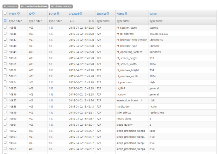
If you are reading this on a fairly large screen or print-out, you may be able to read the name and value of variables that were logged. The ‘Created’ column tells you to the second when the variable was logged. Other columns, from left to right are, ‘Index’, ‘Type’, ‘ID’, ‘Script’, and ‘Subject’. ‘Index’ is a number that uniquely identifies the row of data in the entire NeuroTask database. ‘Type’ and ‘ID’ will be discussed below. ‘Script’ is the id number of the script that generate the data. ‘Subject’ is an index number assigned to each anonymous subject. (The ‘Invite’ column is shown here in older screen shot, but is suppressed at the moment; it may be active again in the future after we have redeveloped the invite and tracking system.)
In this particular data table, you can see that the survey was taken by two subjects with numbers 727 and 734. Both are anonymous, which you can find out by clicking on them: their labels will read ‘anon727’ and ‘anon734’, which is the default labeling system for anonymous subjects.
What a ‘session’ is
We did not yet discuss the ‘Type’ and ‘ID’ columns. ‘Type’ refers to the level at which you are logging data. By default, you are logging data at the ‘session’ level: one ‘subject’ W was doing an experiment with ‘script’ Y written by ‘author’ (i.e., user) Z. The same subject, may use his or her invite link again to take the experiment for the second time. The ‘subject’, ‘script’, and ‘author’ will be the same but the ‘session’ will now be different: Once an experiment has been completed the session is closed.
What if a session has not been closed? If a subject stops doing an experiment midway, the experiment ‘session’ is not closed. If the subjects continues after a while, data is added to the same session. This is the meaning of ‘session’ you see in the ‘Type’ column. One subject can participate in several consecutive sessions: after completing the experiment, he may sometimes decide to do it again (e.g., to get a better score). After starting the experiment for the second time, a completely new session will be opened with a new session ID in the data tables.
A session is recognized by the NeuroTask Scripting system only if the subject continues on the same computer, using the same internet browser. The reason is that the NeuroTask Scripting system leaves so called session cookies behind and these are located in the browser’s database on a specific computer.
When does the system decide the session has to be closed, even though the subject has not finished it? We have set this period at 48 hours, meaning that a subject has two days to get back to the experiment to finish it. After that, an entirely new session is started. So, if a subject starts an experiment on Monday, is interrupted and only gets back to it on Friday (by clicking the experiment URL again), the old session will be closed and the experiment will be treated as a new experiment session.
7.4 Data storage and retrieval
Suppose, your experiment consists of two parts, say a memory task followed by a sleep survey. A subject does the memory task but then needs to do something else and turns off her computer. Later that day she remembers she still need to finish the survey part, turns her computer back on and surfs back to your experiment. To her great annoyance she has to do the memory task again and she decides not to bother with the experiment anymore. How can you prevent this situation?
Above, when discussing what a session is, we said that a session remains open for 48 hours, giving a subject to return to it within two days (even an anonymous subject). But how do you know whether a subject has already completed a section of your experiment? For this, we use store() and retrieve().
The store() function works very similar to the log() function with one great difference: It always overwrites earlier values stored with the same name. The log() function always adds a new row, the store() function adds new rows only if it is storing a value with a certain ID for the first time. Thereafter, it will keep that row and will update the value in that row. The retrieve() function will retrieve the current value for a certain ID, returning undefined if no row exists yet in the database. Also, the retrieve() will halt the script until the value has been retrieved and then continues. This may sometimes cause a slight delay (less than one second usually).
The store() and retrieve() function allow us to use bookmarks, as follows:
 1 var bookmark;
 2
 3 bookmark = retrieve("Where");
 4
 5 if (bookmark !== "Part 1 Completed")
 6 {
 7     // Here comes the memory task
 8
 9     store("Part 1 Completed","Where");
10 }
11
12 // Here comes the sleep survey
The retrieve() function will return undefined if the variable does not (yet) exist, which will be the case when a subject first starts this experiment. After completing the memory task, the variable ‘Where’ will have the value ‘Part 1 Completed’. This means that the first part of the experiment will now be skipped. You can also use this technique to prevent subjects from doing an experiment twice, though in our experience it is better to allow this and simply not analyze this additional data.
Let’s extend the technique above to more than two parts. We will use a number as a bookmark and increase it as the subject does more parts:
 1 var bookmark = retrieve("Where") || 0;
 2
 3 if (bookmark < 1)
 4 {
 5     text("Press '1'"); // dummy task
 6     awaitkey('1');
 7     store(1,"Where");
 8 }
 9
10 if (bookmark < 2)
11 {
12     text("Press '2'"); // dummy task
13     awaitkey('2');
14     store(2,"Where");
15 }
16
17 if (bookmark < 3)
18 {
19     text("Press '3'"); // dummy task
20     awaitkey('3');
21     store(3,"Where");
22 }
23 text("Experiment completed!");
Here we use a well-known JavaScript idiom to assign a default value to a variable that may have value undefined (or null):
var bookmark = retrieve("Where") || 0;
The ||-operator evaluates the expression from left to right. As soon as it encounters something that evaluates to true it returns that value, or else the last value evaluated. If retrieve() returns undefined2, as it will when the variable does not yet exist, the ||-operator will skip the first part and try the second part, which it then returns.
When a subject does this script for the first time, bookmark is 0 and the first part will be presented. If the subject does task 1 (i.e., press 1) and then closes the webpage, the value of bookmark is stored as 1. On opening the experiment again, the usual Landing Page is shown, but now when subject presses the Start button, he or she skips the first part and is now asked to press 2.
If the subject completes the entire experiment and then returns to it later, he or she will start over from the beginning, as a second experimental session will be created with a new subject. The reason is that the system has no way of finding out whether the same person is doing the experiment again or a friend, relative or other person who has access to the same computer.
The retrieve() function also has a third argument, namely a timeout, which is set to 5000 ms by default. If the retrieve() function does not succeed in retrieving a value from the server within the timeout period, it will return null. You can disable timeout by setting the third argument to 0. But beware, in case the internet connection fails the script will stay stuck and not move forward.
You can check for null and undefined like this:
var x = retrieve("Where");

if (x === undefined) // Note the triple equal sign ===
{
    // Variable is not yet stored
}

if (x === null)
{
    // There was a timeout
}
Storing ‘behind the scenes’ or storing now
There is no timeout period for store() or log(), because these function do their job ‘behind the scenes’. While the rest of your script continues to run, the store() and log() functions are collecting data until they have enough or until no data has come in for a while. Then, they communicate with the server and send the data for processing and storage there. This does not interfere with your script. Just be sure that you do not suddenly have the subject move away from the script (e.g., by redirecting to a survey site) without first calling closesession(), which halts the script until all data has been written to the database. With retrieve(), a value must be retrieved before the script can usefully continue. Therefore, we let the script wait until the value has been secured or until timeout.
If you ever have a situation where you need to be certain for the good operation of your script that a value has with certainty been stored on the server, you can use the store_now() function, which works like store() but blocks further processing until the server has confirmed the correct storage of the variable. (This function stores and does not log the data.)
Storing at the ‘script’ and ‘author’ level
By default store(), store_now() and retrieve() operate at the ‘session’ level. The bookmark above was associated with the current session in the database. It may also be necessary to store variables at the level of the script. For example, you may want to count how many times subjects have done your experiment and use this number in your script to assign a new subject to one of two conditions (e.g., on even count to condition 1). This is achieved by storing variables at the ‘script’ level (always written in lower case).
You can also use this functionality to create multi-player turn-based games. Examples are given at https://scripting.neurotask.com/howto/multiplayer_game and another at https://scripting.neurotask.com/howto/tic_tac_toe_multiplayer_version. Here, the ‘script’ level is used to first have a new player A matched to waiting player B. Both players are given a long random ID string. Now player A can store a game move to that ID, e.g., in a chess game ‘bishop to e5’ could be sent as store_now('Be5','ssefse24948594','script'). After having, thus, ‘sent’ a move by storing it in this manner, the script will keep polling the id to see whether a counter move has been posted. (Or a more elaborate JSON structure may be ‘sent’ where also the sender is identified and the time.) If so, the player is notified and can make a move again. Etc. Each script can have many ‘channels’ in this manner, each linking two sessions.
In some cases, it is useful to store variables at the level of the author, for example, to keep track of information in several different scripts. You can use the ‘author’ level for this. Both ‘script’ and ‘author’ variables can be found via the Scripts menu at Scripts -> Script Data -> Stored Script Variables and Scripts -> Script Data -> Stored Author Variables, resp.
increase() and decrease()
As note above, there may be cases where you want to keep count of something, for example, how often a certain experiment has been done. Or you may want to assign consecutive numbers to your subjects and use these for your own bookkeeping. For this purpose, we have included the increase() function, which like store_now() will wait for a confirmation and then return the increased value. You can use it like this:
var subject_id = increase("Subject ID","script");
If the variable ‘Subject ID’ does not yet exist, it will be inserted into the data table with starting value 0 plus your initial increase value, which is 1 by default. If it exists, the value of the variable will be increased. This only works with (signed) integers. You can increase with a greater step size, by specifying this as a third argument, e.g., increase("Total_failed","script",failures) to update the total number of failures recorded (e.g., subjects failing a certain test).
So, if this would be the very first time the script is run by any subject, subject_id would receive the value 1. On each subsequent run, the return value would be 1 higher. Also, the ‘Subject ID’ variable in your data table would reflect how many subjects have done your experiment.
The decrease() function works completely similar to increase(), except that the specified amount is decreased from the current value. Note that both increase() and decrease() have default timeout periods of 5000 ms, which can be adjusted by adding a fourth argument (e.g., 10000 for 10 s or 0 if you want no timeout at all, see comments above), e.g., increase("Total_failed","script",failures,2000).
7.5 Working with the data tables
In this section, we will go over a few tricks for working with data tables. Note that these are not just used for session data, but also to present overviews of subjects, invites, and scripts. All of these can be downloaded to Excel and other formats and managed as described below. We will here focus on how to manage data collected in an experiment, but the principles are similar if you want to say manage the overview table in which all subjects are listed.
If you go to a script and then click on the table icon, you will see all data collected by that script during experimental sessions; each time log() was called another row was added to the table. If you have many subjects taking your tests and if you collect much data per script, this may result in thousands of rows. Fortunately, the data tables offer several ways to make inspection of your data more manageable, notably sorting and filtering.
Clicking on one of the headers (Type, ID, etc.) will sort the table according to that column. By default only 20 rows are shown, but in the Rows menu at the bottom, you can set this as high as 320. Next to the Rows menu, at the bottom of the table, is the Columns menu. There, you can uncheck the columns you are not interested in at the moment. These will be hidden from view and, if you wish, may be excluded from a download.
To alert you to any hidden rows and columns (lest you forget you had hidden these), at the very top of the table, the number of hidden rows and columns (if any) is given in the blue field above the column. If there are not hidden rows or columns, these fields turn grey.
Filtering data
Each column in the tables has a so called ‘filter’ option, which allow you to hide certain rows. Below the column header is a field that says ‘Type filter’ in pale grey letters, where you can type a ‘search’ text. You could, for example, type 'nt_' in the filter field of the ‘Name’ column. Any row of which the variable name contains 'nt_' somewhere (not necessarily at the beginning) will be shown and all other rows will be hidden. The number of rows hidden is shown in the blue field at the top-left of the table. The 'nt_' variables are the ones that are collected automatically. If you want to hide those rows, e.g., to focus on your own data, you must put an exclamation mark at the beginning, which in many computer languages, including JavaScript, means opposite or negation. So, you would enter '!nt_' in the filter field. By planning ahead a little with the names you give to your variables, you could make good use of these filter options. For example, you could filter on 'cond1' or 'cond2', or have summary variables like 'summary_test1', 'summary_test2', where you could filter on 'summary_' to get a quick overview.
For advanced users, there is even the possibility to use regular expressions as filters, if you start a filter text with a question mark it is interpreted as a regular expression. Regular expressions are quite powerful but hard to learn and their usage here is beyond the scope of this introductory manual. As an example: ‘?e$’ would show all names ending in ‘e’. And '?nt_|rt_' would show all values that contain either 'nt_' or 'rt_' (or both).
In the a date column, such as the Created column, you can filter among others by ‘days ago’. Today’s data can be shown with '0..1' (two dots). Last week’s data, including today, with '-7..1' and so on. Decimals are allowed to if you want say the last few hours. You can also click on the > < symbols, which will present you with calenders where you can select the ‘from’ and ‘to’ dates you wish to inspect.
In numeric fields, such as the Script (ID) column, you can use ranges as well, such as 1000..1200. Or !1000..1200 to exclude this range. Just typing say 1023 will show only the data of the script with ID 1023.
Finally there is the checkbox filter, which has values ‘indeterminate’ (which is the default, meaning it is not active), ‘checked’ where only the checked rows are shown, and ‘unchecked’ where only the unchecked rows are shown.
All of these filters not only change your view of the table by hiding certain rows, the view achieved by them can also be exported, if you want that.
7.6 Exporting data
If you scroll all the way down below the table, you see a title bar that says ‘Excel or CSV Export’. Clicking on brings up an image like this:
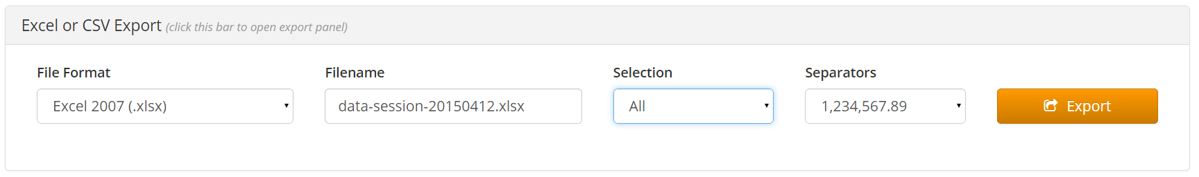
In the File Format menu on the left you can select the type of file you want to download:3
- Excel 2007
- Excel 5
- CSV (plain text with comma-separated values)
- HTML (web page)
With the Selection menu you specify which ‘view’ of the table you wish to download:
- All
- Filtered
- Checked
‘All’ gives you all rows. Filtered gives you only the visible rows and columns. This is handy if you want to download a specific portion of your data. Checked will export only the columns that you checked by clicking the checkboxes on the very left-hand side. This is useful for very specific selections of rows.
The Separators menu is relevant if you want to export your data for use in a translated (non USA English) version of Excel, such as Dutch, which uses the comma for a decimal sign and the point to separate thousands.
In the menus at the bottom of the data table, you can also find three Quick Export options. These do not run via the NeuroTask server, but work locally, in the browser. They only produce Excel and the formatting is somewhat atypical. You can use it as a fallback in case there is a problem with the regular exporting facility, such as a sudden internet connectivity problem.
Because the data table is quite sophisticated in its filtering capacities, it becomes very slow and memory hungry for large data sets. If you have collected more than 100,000 data points (i.e., rows), this page will automatically redirect to data_alt which has only limited export possibilities. For this reason it is better to use the datadashboard, which also is much better suited to export data in a format suitable for subsequent import into SPSS and Jasp. It also allows filtering, if you first go to the ‘filter page’ via the Scripts menu: Scripts -> Script Data -> Prefilter Data for the Data Dashboard. There you can retrieve only data for one subject, or collected since so many days ago (e.g., to analyze the latest data), or of only a single named variable. The data dashboard will be discussed in more details below.
Pivot tables, or how to make your tables ‘square’ again
Some users may wonder about our choice to store all data in a big table with many rows and few columns. Wouldn’t it be handier to have a square table with say the subjects as rows and their data as columns. With thought very hard about this and our conclusion was: No, this is not handier except in certain specific case. The format we use is the least limiting format, because of one extremely handy tool: pivot tables. These are present in all Excel programs and we strongly encourage you to spend one or two hours familiarizing yourself with them.
A pivot table turns a long table like you download from NeuroTask Scripting into an arbitrary square table with summary statistics such as ‘count’, ‘mean’, and ‘standard deviation’. You can format an Excel pivot table in minutes, using dragging and dropping of fields. For example, suppose you have this:
| x | y |
|---|---|
| 1 | 2 |
| 1 | 4 |
| 2 | 3 |
| 2 | 6 |
x could be subjects IDs and y a percentage correct on certain trials or reaction times.
With a pivot table we can take the mean value over all repeated measurements in conditions 1 and 2, which would give us this:
| x | mean |
|---|---|
| 1 | 3 |
| 2 | 4.5 |
What an Excel pivot cannot do is to turn the long table into a square with textual and other values; you are forced to use numeric values and summary statistics as values of the pivot table (but not of the row and column headers).
7.7 Logging, storing, and the ‘response’ object
Data which is collected with the log() or store() functions is always also available in the response object. So, if in your script you write:
log(391,"average_rt");
The value 391 can be accesses in the response object, e.g.,
var save_for_later = response['average_rt'];
More useful is the fact that each string in NeuroTask Scripting has a format() function, which can take the response object as an argument, such that its key-value pairs can be used in a string, as follows:
var s = "Your reaction time was {average_rt} ms".format(response);
Now string s will be equal to ‘Your reaction time was 391 ms”. As is explained in the chapter on form controls, each of these controls already does this by default, so that earlier responses can be used in the labels and explanatory text of these controls.
7.8 Deleting data
In the Scripts -> Script Data menu, there is also an item marked with a red cross that says Page for Deleting Logged Data. At that page, you can delete logged data either for a specific subject, a specific logged event (for all subjects), or you can delete all logged data for the script. Deleting data may be desirable for security reasons and because of ethical considerations. Needless to say: be very careful with this. Data deleted in this manner can no longer be retrieved, not even by the NeuroTask Scripting staff!
7.9 Data Dashboard
The data dashboard, shown in the button bar with the  data dashboard icon, is now the default way to view and export your data. It is much faster than the other data exports and can handle much larger files: we have tested Excel exports to files with up to 900,000 rows of data (using Firefox on Windows). To take full advantage of its capacities, it is necessary to log your data with the appropriate conditions. This works as follows.
Suppose, you are doing a lexical decision reaction time experiment with one dependent variable, called ‘RT’ (reaction time in ms). There are two conditions. ‘Condition 1’ is showing long or short words to which the subject must respond with ‘Word’ (press ‘s’ key) or ‘Non-Word’ (press ‘l’ key) as fast as possible. ‘Condition 2’ is whether it is in face a word or not. We can now log the ‘RT’ variable with the conditions as follows. (We have here entered some random RT values a particular subject might have.)
logtrial(120,"RT","short","word");
logtrial(150,"RT","short","nonword");
logtrial(130,"RT","long","word");
logtrial(200,"RT","long","nonword");

logtrial(160,"RT","short","word");
logtrial(165,"RT","short","nonword");
logtrial(170,"RT","long","word");
logtrial(180,"RT","long","nonword");
Here, we have simply entered some values for the reaction times; normally these would be obtained from actual subject responses. From left to write we have: value, variable name, conditions. If we run this experiment so that the data are stored and move to the data dashboard, we see something like:
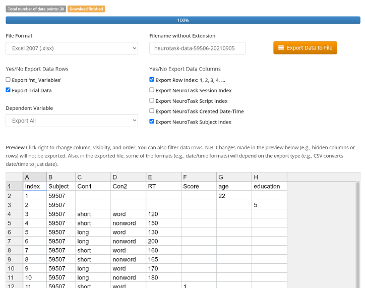
logtrial().The conditions are indicated as ‘Con1’, ‘Con2’, … You can have as many conditions as you want but you cannot at present name them yourself. The dependent variable, however, will keep its own name. Now, this format can be imported easily into SPSS, JASP or some other analysis program.
You can still store one-off variables (e.g., age, education, gender, …). E.g.:
logtrial(22,"age");
This usage and its effect are identical to the log() function:
log(22,"age");
It is possible to store many different dependent variables with the same or different conditions:
logtrial(120,"RT","short","word");
logtrial(1,"Accuracy","short","nonword"); // 1 correct answer
Both dependent variables will now be available, each in their own column, though you are also able to select just one variable via a dropdown select.
The logtrail() function is merely a ‘convenience’ function that translates the above into:
log(120,"RT/short/word");
log(1,"Score/short/nonword"); // 1 correct answer
The /-notation used with log() gives identical results to the logtrial() function and you can use either; there is no real reason to prefer one over the other apart from convenience.
The data dashboard has a preview table to give you an idea of your data and options to show/not show data index, subject ID, etc. You can also hide the trial data (i.e., that stored with logtrial()), export only nt data (with technical properties of subjects’ browsers), only data from one condition, etc.
There are many export formats available, some quite arcane. The page may have some initial delay while it is setting up the download. For long downloads the progress can be followed in the progress bar. Once the data have been downloaded to the page, exports are very fast and do not require additional server access; they are generated in the browser.
In case you are mainly collecting survey data, the data dashboard format is less convenient, perhaps, and you may prefer the other data page.