Chapter 2: Type Construction

In this chapter: * house of cards * algebraic data types * Maybe yes, maybe nothing * Lists and recursive types * Function definition

You got to the “Nobu” right on time, barely past seven. As you were approaching the hostess, a hurricane of a girl ran into you - “Thank goodness you got here on time, Curry!” - Curry, that must be my name? But why, I don’t even like curry?! Must be a different reason… - grabbed your hand and dragged you past the busy tables somewhere deep in the restaurant, through the kitchen, out the back door, down the stairs, and into a dimly lit room. In the middle of the room stood a card table - green cloth, some barely visible inscription that spelled “Monoid” in golden letters on it, - surrounded by six massive chairs that looked really old. The girl abruptly stopped, turned around, looked you right in the eye - hers were green - and asked almost irritably, but with a pinch of hope in her voice:

– Well? Are you ready?
– Ahem… Ready for what?! Can you explain what’s going on?
– Did you hit your head or something? And where were you last week? I called like 27 times! And why do you smell like manure - did you suddenly decide to visit a farm?! Ah, no time for this! - she dragged you to the table and pushed you into one of the chairs - she was strangely strong despite being so miniature - so that you had no choice but to sit. BOOM! Suddenly, a small fireworks exploded in your eyes, and you felt more magic coming back to you.

Out of thin air, you create a new deck of cards with intricate engravings on their backs, nothing short of a work of art. You feel them - they are cold and pleasant to touch, - but then rest your hands on the table, close your eyes, and.. it’s as if the cards became alive and burst in the air above the table, shuffling, flying around, dancing. You open your eyes, enjoying your newly mastered power over cards, barely nod your head, and the deck, obeying your wishes, forms into a fragile house of cards right beside the Monoid sign.

You turn to look at your mysterious companion. She is smiling and there are twinkles in her eyes.

House of cards with a little help from Algebra

Looks like our mage is making friends and remembering new spells, this time without risking any animal’s wellbeing. Let’s follow in his footsteps and learn some card magic!

First, try dealing some cards in our repl. Just follow the link and click “run”. You’ll see some beautiful (well, not as beautiful as the ones Curry created, but still..) cards being dealt: … 9♥ 10♥ J♥ Q♥ K♥ A♥ - with barely more than 20 lines of code. Let’s understand what’s going on here step by step.

To start doing card magic - or card programming for that matter - we also need to create a deck of cards out of thin air. Here’s one way of doing it in Haskell:

 1 -- Simple algebraic data types for card values and suites
 2 -- First, two Sum Types for card suites and card values
 3 data CardSuite = Clubs | Spades | Diamonds | Hearts deriving (Eq, Enum)
 4 data CardValue = Two   | Three  | Four     | Five  | Six  | Seven | Eight |
 5                  Nine  | Ten    | Jack     | Queen | King | Ace
 6                  deriving (Eq, Enum)
 7 
 8 -- Now, a Product Type for representing our cards:
 9 -- combining CardValue and CardSuite
10 data Card = Card CardValue CardSuite deriving(Eq)

We have created three new types above. CardSuite is inhabited by 4 values: Clubs, Spades, Diamonds and Hearts - just like Int is inhabited by 2⁶⁴ values - that correspond to playing card suites. CardValue is inhabited by 13 values that represent card face values. All of it is pretty self-explanatory. Type Card represents a specific card and is a little bit more interesting - here we are combining our two existing types into one new type. Don’t mind deriving statements for now - we’ll explain them down the road, suffice it to say that here Haskell automatically makes sure we can compare values of these types (Eq) and we can convert them to numbers (Enum).

Open the repl linked above again, run it (if you don’t run it first you’ll get an error as the types won’t be loaded into the interpreter), and then play with these types on the right:

 1 > let val = Jack
 2 > val
 3 => J
 4 > let suite = Spades
 5 > suite
 6 => ♠
 7 > let card = Card Ace Hearts
 8 > card
 9 => A♥
10 > let card1 = Card val suite
11 > card1
12 => J♠

Here we bound val to CardValue Jack, suite to CardSuite Spades and created 2 cards - Ace of Hearts directly from values and Jack of Spades from our bound variables - both approaches are perfectly valid. Create some other cards in the repl to practice.

Looking at the types definition above, the syntax for type creation should become apparent: to create a new type in Haskell, we write data <Name of Type> = <Name of Constructor1> <Type of value 11> ... <Type of value 1n> | <Name of Constructor2> <Type of value 21> ... <Type of value 2m> | ... . You can read symbol | as “or” - it is used for combining different types together into a new Sum Type, values of which can be taken from a bunch of different types we are combining, but every value is taken from only one of them. Types like data Card = Card CardValue CardSuite are called Product Types, and every value of such type contains values of all of the types we are combining.

Algebraic Data Types

Sum and Product types together are called Algebraic Data Types, or ADT in short (which may be confused with abstract data types that are quite a different matter, but we will call algebraic types ADT), and they form a foundation of any modern type system.

Understanding ADTs is extremely important in Haskell programming, so let’s spend more time discussing them and looking at different ways to define them. Here are several more examples.

Type Person, containing their name and age: data Person = Person String Int. We are combining a String to represent a name and an Int to represent an age, and then we can create people like so: Person "Curry" 37 or Person "Jane" 21. This is a product type.

What if we wanted to represent built-in JavaScript types in Haskell - String, Number, Date, Object, etc? Here is one way of doing it (it does not allow us to represent everything, we will look at the full javascript values type definition once we learn recursion):

1 data JSValues = JString String | JDate Int | JNumber Double | Undefined

Now, this is interesting - we have combined three types that “store” a String, an Int and a Double inside a constructor and add a simple value “Undefined” as the fourth possible value. It means that values like JString "hello world", JDate 12345225 (which is quite a long time ago), JNumber 3.141 and Undefined are all valid values of the type JSValues. This is a sum type.

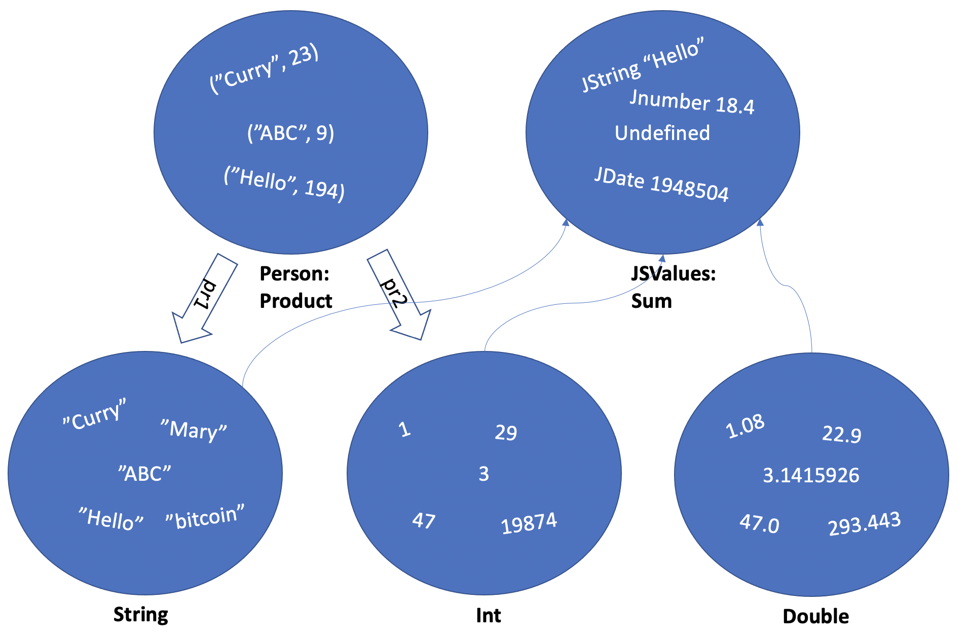
By now, you should get a pretty good feel on what sum and product types are. When you create a product type, you combine values of several different types in one value, represented as a tuple $(x_1:t_1, x_2:t_2, ... )$. When you create a sum type, each value of your type can be from a different type, but only one.

Records

What if you wanted to extend the type Person to include more information about a person, which would be much more useful in the real world situation? E.g., place of birth, parents, first and last names, education, address etc. If you had to write something like

1 data Person = Person String String Int Date Address Person Person
2 
3 jane = Person "Jane" "Doe" 25 (Date 12 10 1992) addr father mother

it would be extremely confusing to use - you’d need to remember the order of fields, you’d confuse fields with the same types etc. Thankfully, Haskell supports records - basically, a Product Type with named fields. We can define our Person type properly like this:

 1 data Person = Person
 2   {
 3     firstName :: String
 4   , lastName  :: String
 5   , age       :: Int
 6   , dob       :: Date
 7   , address   :: Address
 8   , father    :: Person
 9   , mother    :: Person
10   }
11 
12 -- you can still initialize a record just by applying a Constructor ('Person') to a \
13 bunch of values in order
14 jane = Person "Jane" "Doe" 25 (Date 12 10 1992) addr mother father
15 -- ... or, you can access the record's fields separately by their respective names
16 janesSister = jane { firstName = "Anne", age = 17, dob = Date 1 1 2000 }

Before we move on to the other ways of constructing new types, here is yet another example, which illustrates how Product and Sum types work together. Let’s say we want to model different 2-dimensional geometric shapes. We can define the following Product types:

1 data Point = P Double Double -- x and y
2 data Circle = C Double Double Double -- x and y for the center coordinates, radius
3 data Rectangle = R Double Double Double Double -- x and y for the top left corner, w\
4 idth and height

Now, let’s say we want a function that calculates the area of our shapes. We can start like this:

1 area :: Rectangle -> Double
2 area (R x y w h) = w * h
3 -- since we are not using x and y values from our Rectangle to calculate the area, w\
4 e can omit them in
5 -- our pattern match like so:
6 area (R _ _ w h) = w * h

This works fine. But we need to calculate the area of Circles as well, and potentially other shapes. How do we do it? If you try to define another function area :: Circle -> Double the typechecker will complain because you already have a function named area that has a different type. So what do we do? Create a differently named function for every type? Now, that would be ugly!

There are several approaches to solving this. (This is actually one of the problems with Haskell - you can solve one task in many different ways, there’s just so much power and flexibility that sometimes it is getting overwhelming, and not just for beginners. We will see many examples of this down the road). One of them is using Typeclasses, another one - using Type Families (probably overkill in this case) - we’ll get there soon. But now we will simply use a Sum Type. We can combine three of our shapes (product types) into one sum type. There are actually two ways to do it! The first one is if we want to keep Rectangle, Circle, and Point as separate concrete types in our system. Then we will use the definition above and will combine them into one type like so:

1 data Shapes = PointShape Point | CircleShape Circle | RectangleShape Rectangle

Then, our area function can be defined as follows with the help of pattern matching:

1 -- notice the type signature change:
2 area :: Shapes -> Double
3 -- we don't care about the point coordinates, area is always 0 
4 area (PointShape _) = 0 
5 -- notice the nested pattern match below:
6 area (CircleShape (C _ _ r)) = r * r * pi
7 area (RectangleShape (R _ _ w h)) = w * h

Now everything will work like a charm. When you write somewhere in your code area myShape it will check which exact shape is myShape - Point, Circle or Rectangle - and will choose the respective formula.

An alternative way to achieve the same result is to define Shapes type directly as a Sum Type like so:

1 data Shapes = Point Double Double | Circle Double Double Double | Rectangle Double D\
2 ouble Double Double

I leave the area function definition for this case as an excersize. The difference with the previous approach is that in this case you will not have types Point, Circle and Rectangle in your type system - they are simply constructor functions now. So trying to define a function from Rectangle to Double will be a typechecker error.

Using Sum and Product types you can express a lot of real world modeling already, but why stop there? We want to be even more efficient and polymorphic! Read on.

Type Functions Are Functions, Maybe?

Let’s spend some time reviewing a statement we made in the last chapter: type and data constructors are functions. This is extremely important to understand and internalize, so that you do not become confused when writing real world programs that use monad transformer stacks and similar concepts that may look overwhelming, but are in fact quite simple. You need to be able to easily read type signatures and understand their structure at first glance.

Let’s look at a couple of types, renaming type names now to distinguish between types and constructors: data Cards = Card CardValue CardSuite and data People = Person String Int. The part on the left is the name of the type, the part on the right is the name of the data constructor and types of the values that this constructor contains. So, in reality Card is a function that should be read in Pascal-ish pseudocode as function Card (x:CardValue, y:CardSuite) : Cards - i.e., it’s a (constructor) function from 2 variables, one of type CardValue, another of type CardSuite that returns a value of type Cards! Same with Person, which turns into function Person (x:String, y:Int) : People.

In fact, using so called GADT (generalized algebraic data types) Haskell notation, this becomes even more apparent - below is the solution to the task of extending Card type with the Joker card written first with the familiar syntax and then using GADT:

1 data Cards = Card CardValue CardSuite | Joker
2 
3 -- same using GADT
4 data Cards where
5   Card  :: CardValue -> CardSuite -> Cards
6   Joker :: Cards

Looking at the 2nd variant, the point about Card and Joker being functions becomes much clearer. In effect, it tells us that we are defining type Cards which contains 2 constructors: Card, which takes 2 arguments of type CardValue and CardSuite and returns a value of type Cards, and Joker, that takes no arguments (or strictly, an empty Type - ()) and is a value of type Cards.

We can take it one step further, and take the analogy of Product and Sum types to it’s fullest - we can treat the type Cards as type function that is a sum of 2 product types: typeFunction Cards = Card (x : CardValue, y : CardSuite) + Joker()! Of course + here has nothing in common with arithmetic sum but has the same meaning as | in real Haskell syntax.

So, Card is a constructor that creates a value of type Cards from 2 other values, and Cards, even though we just called it a type function, is in fact a “type constant”. It is a concrete type - you cannot apply it to another type and construct a new one. Unlike type function List that we hinted at in the last chapter, that actually creates new types from other types - and as such is much more interesting and important for us. We’ll get to it in the next section and we’ll need to understand it to follow along our card dealing program further.

For now, let’s start with the simplest real (non-constant) type function, one that constructs new types from other types: Maybe, which is used ubiquitously in Haskell.

1 data Maybe a = Just a | Nothing
2 
3 -- in GADT syntax:
4 data Maybe a where
5   Just    :: a -> Maybe a
6   Nothing :: Maybe a

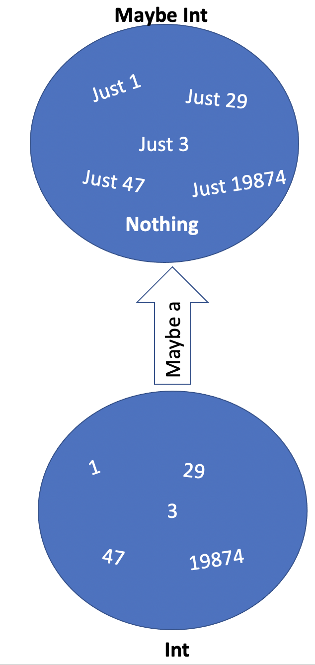
This notation is very often a source of confusion for beginners and even advanced Haskell students - we are using variable a on both sides of the type definition, but they mean very different things on the left and on the right! In fact, this confusion should be cleared if you read this sort of definition in the spirit of what we’ve described above: typeFunction Maybe (a : Type) = Just (x : a) + Nothing (). Please dwell on it until you fully understand the issue - it will save you lots of hours of frustration with more complex types down the road. We are in effect saying here: Maybe is a type function that takes a type variable a and creates a new type from it (Maybe a) with help of 2 constructor functions - Just, that takes a “regular” variable of type a and creates a value of type Maybe a, and Nothing, a function of zero arguments that is a value of type Maybe a. So, a is a variable of type “Type” - it can take a value of any Type we defined - on the left, and it is used in the type signature for constructor function Just variable on the right.

Take a breath and let it sink in.

Why is the type (which really is a type function) Maybe a useful? It’s the easiest way to handle failure in your functions. E.g., you could define a function divide like so:

1 divide :: Double -> Double -> Maybe Double
2 divide x 0 = Nothing
3 divide x y = Just (x / y)

This function would return Nothing if you try to divide by zero, instead of crashing or throwing an exception, and Just <result of division> if you divide by non-zero. This is a trivial example, but Maybe is of course very useful in thousands of other more complex situations - basically, anywhere you need to handle possibility of failure, think about Maybe (there are other ways to handle failure and errors in Haskell as we shall see further on).

Note also function definition syntax - a very powerful and concise pattern matching approach. Under the hood, this definition translates into something like:

1 divide x y = case y of
2                       0 -> Nothing
3                       _ -> Just (x/y)

.. but in Haskell you can avoid writing complex nested case statements and simply repeat your function definition with different variable patterns, which makes the code much more readable and concise.

So, what if we also have a function square x = x * x that works on Doubles and need to apply it to the result of our safe divide function? We would need to write something like:

1 divideSquare x y = let r = divide x y in
2                    if r == Nothing then 0
3                    else <somehow extract the value from under Just and apply square \
4 to it>

To do the “somehow extract” part in Haskell, we again use pattern matching, so the function above would be written as:

 1 -- function returning Double
 2 divideSquare x y = let r = divide x y in
 3                    case r of Nothing -> 0
 4                              Just z  -> square z
 5 
 6 -- or, better, function returning Maybe Double as returning 0
 7 -- as a square of result of divide by zero makes no sense
 8 divideSquare x y = let r = divide x y in
 9                    case r of Nothing -> Nothing
10                              Just z  -> Just (square z)

We pattern match the result of divide and return Nothing if it’s Nothing or Just square of the result if it’s Just something. This makes sense, and we just found a way to incorporate functions that work between Doubles into functions that also work with Maybe Doubles. But come on, is it worth such an complicated verbose syntax?! Isn’t it better to just catch an exception once somewhere in the code and allow for division by zero?

Yes, it is worth it and no, it’s not better to use exceptions, because you can rewrite the above as simply divideSquare x y = square <$> divide x y, or looking at all the function definitions together:

 1 square :: Double -> Double -> Double
 2 square x = x * x
 3 
 4 -- safe divide function
 5 divide :: Double -> Double -> Maybe Double
 6 divide x 0 = Nothing
 7 divide x y = Just (x / y)
 8 
 9 -- our function combining safe divide and
10 divideSquare :: Double -> Double -> Maybe Double
11 divideSquare x y = square <$> divide x y
12 
13 -- compare with the same *without* Maybe:
14 divide' x y = x / y -- will produce an error if y is 0
15 
16 divideSquare' :: Double -> Double -> Double
17 divideSquare' x y = square $ divide' x y

Wow. Isn’t it great - we are using practically the same syntax for both unsafe functions between Doubles and safe functions between Maybe Doubles, and what’s more, we can use the same approach for a lot of other different type functions, not just Maybe a.

Here, operator $ is just function application with lowest precedence, so allows to avoid brackets – without it you’d write square (divide' x y) – and <$> is another operator that also applies functions defined for concrete types, but it does so for values built with special class of type functions from these types, e.g. Maybe a or List a - without the need to write nested case statements. It is a key part of something called a Functor in both Haskell and Category Theory and we will look at it in more detail in the next chapter.

In the end, it’s all about making function composition easy - remember Chapter 1 and how to think about solving problems functionally? You break the problem down into smaller parts and then compose functions together, making sure input and output types “fit together”. All the complicated scary terms you may have heard or read about in Haskell - Functors, Monads, Arrows, Kleisli Arrows etc - they are all needed (mostly) to make composing different functions easy and concise, which, in turn, makes our task to decompose a problem in smaller pieces so much more easy and enjoyable. So don’t be scared, it will all make perfect sense.

Advanced: On Data Constructors and Types

It pays to understand how Haskell (GHC specifically) treats and stores values of different types. One of the powerful features of Haskell is that it is a statically typed language - which means there is no type information available at runtime! This leads to much better performance with at the same time guaranteed type-safety, but is a source of confusion for many programmers coming from the imperative background.

Let’s look at the type Person we defined above, changing the names a bit to avoid confusion:

1 data Person = PersonConstructor String Int 
2 
3 -- or, in a clearer GADT syntax:
4 data Person where
5   PersonConstructor :: String -> Int -> Person

The name of the type is Person and it has only one data constructor called PersonConstructor that takes an Int and a String and returns a “box” of them that has a type Person. Technically, it creates a tuple (n :: String, a :: Int) - so for instance when you write something like john = PersonConstructor "John" 42 you get a tuple ("John", 42) :: Person. The beauty of Haskell is that during type checking stage the compiler has only one job - make sure your functions compose - i.e., input types to all the functions correspond to what the function expects, an output type of all the functions corresponds to their type as well. Once this check is done - all the type information gets erased, it is not needed, as we have guaranteed and proved it mathematically that every function will receive correct values at runtime. This immensely increases performance.

So, if you have a function showPerson :: Person -> String that is defined something like showPerson (PersonConstructor name age) = name ++ " is " ++ show age ++ " years old" and then you call it on John person from above, here is what happens:

1 st = showPerson john
2 -- gets expanded into:
3 showPerson (PersonConstructor "John" 42)

Under the hood it is simply a tuple (“John”, 42), and according to the pattern match on the left side of showPerson definition we get name = "John" and age = 42. Then these values get substituted in the function body and we get a resulting string. But nowhere is type Person used! Typechecker gurantees that the first value in a tuple received by showPerson will have type String, while the second - Int, so it is impossible to have a runtime error!

In a general case, if you have a data constructor <Cons> T1 T2 ... TN that belongs to some type MyType and then when you call it to create a value as <Cons> x1 x2 ... xn - Haskell stores it as a tuple (x1,x2, ..., xn) of type MyType. The type is used during type-checking stage and then gets erased, while type-safety is guaranteed by math.

For sum types, the situation is a bit trickier. Recall our type of Shapes:

1 data Shapes = Point Double Double | Circle Double Double Double
2 
3 area :: Shapes -> Double
4 area (Point _ _) = 0
5 area (Circle _ _ r) = pi * r * r

It has in this case two data constructors - Point and Circle, which behave exactly as described above. Function area during compilation gets re-written using case-analysis, in pseudo-code:

1 area (s :: Shape) = case <constructor of s is> of
2     Point -> 0
3     Circle -> <get 3rd element of the (x,y,r) tuple and substitute for r in pi * r *\
4  r>

This means that for sum types of more than one data constructor Haskell needs a way to distinguish between data constructors with which this or that tuple has been created. So, even though information that s is a Shapes type is erased, we keep the constructor number inside the type together with our tuple. So that Point 4 0 would be represented something like (0, 4, 0) (in reality it’s done differently, but this illustrates the concept well enough) where first value of the tuple is the constructor tag. GHC uses a lot of very smart optimizations under the hood where this approach has minimal possible overhead at runtime as well.

List, Recursion on Types and Patterns

Let’s come back to our card-dealing magic spells, available in the repl here. To (almost) fully understand it, there’s only one extremely important piece missing: List type function and recursively defined types, which are extensively used in functional programming to implement various data structures. If you recall, in Chapter 1 we described List as some manipulation that takes all possible ordered combinations of values of another type and creates a new type from it. Try to define the List type function yourself before reading further.

Here is how we can operationalize this definition:

1 data List a = Cell a (List a) | Nil
2 
3 -- or, in GADT syntax:
4 data List a where
5   Nil  :: List a
6   Cell :: a -> List a -> List a

Remember how you need to read type definitions as type functions? In pseudocode: type function List (a : Type) = Cell (x:a, y: (List a)) + Nil() – List a is a type function from the variable a : Type, or a : * in real Haskell, that consists of 2 constructors: Nil, that is itself a value of type List a, and Cell, that takes a value of type a and a value of type List a (here is where recursion comes into play!) and returns another List a. Here Nil is the boundary case of our recursion, and Cell is a recursive function that constructs a list until it is terminated by Nil value as the last element.

Let’s construct a list from values 1, 2 and 3. You have a constructor function Cell that takes 2 values - a value of some concrete type, in this case an Int, and a List of Int. What is the simplest List? Of course it’s a Nil! So, we can write Cell 3 Nil - and it will be a List Int! Now, we can pass this list to another Cell call, like this: Cell 2 (Cell 3 Nil) - and we have yet another List Int. Apply it one more time, and you get Cell 1 (Cell 2 (Cell 3 Nil)). Easy, right?

Basically, if you keep in mind that type functions and constructors are, well, functions, which follow all the same principles as “real” functions, this type building business should become very clear and easy for you.

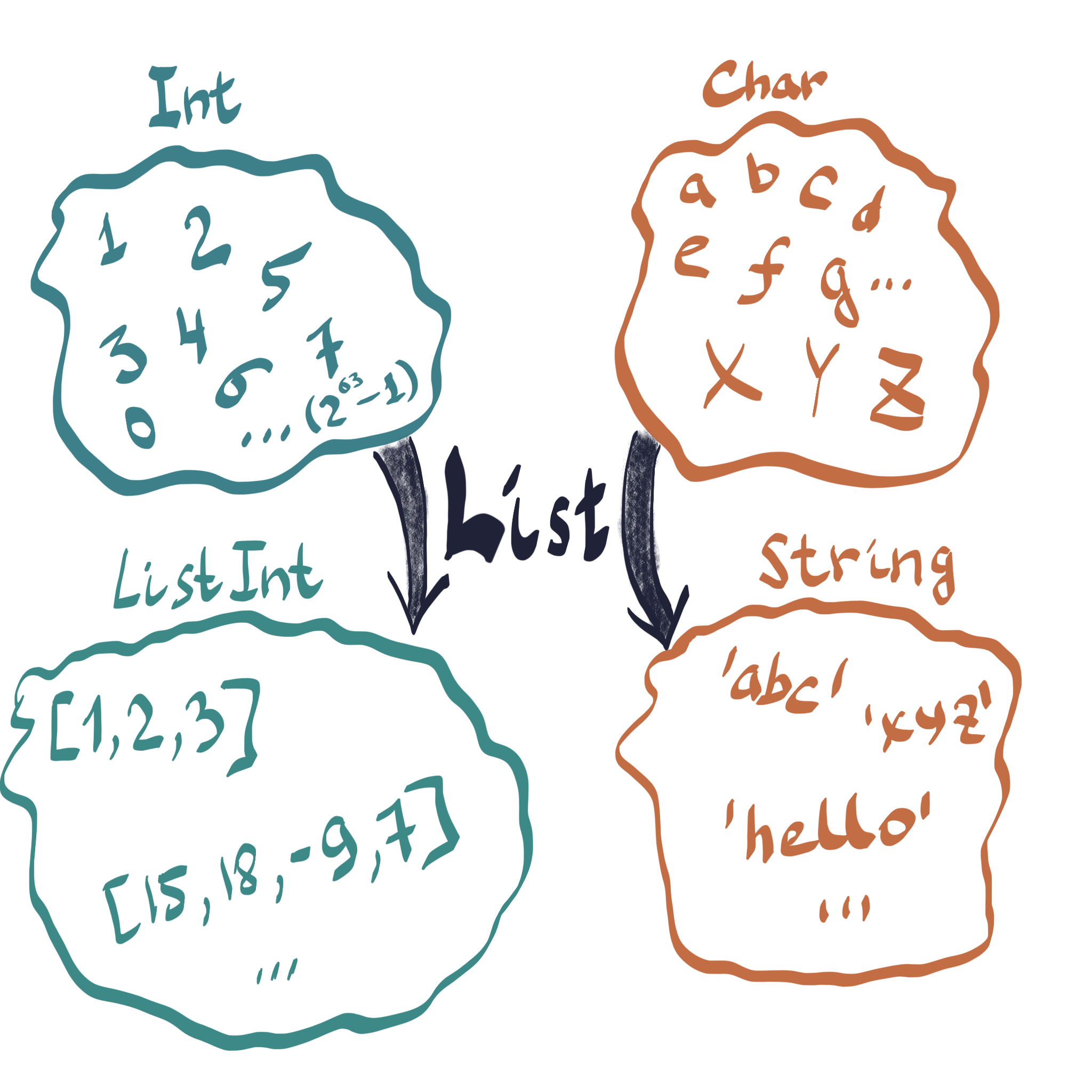
We looked at the principle of how List a type function can be defined, but since in Haskell it is such a fundamental data structure, it is in fact defined with different constructor names and some syntactic sugar on top: Nil is in fact [] and Cell is defined as an operator :, so that our list of 1,2 and 3 would be written as 1:2:3:[] or simply [1,2,3] - much more concise and convenient. You can write ["abc", "hello", "world"] - a value of type List String, or [1.0, 3.1415926, 2.71828] - List Double, etc.

In the last chapter we introduced the type String as a set of all possible ordered combinations of characters, or simply List Char. In fact, it is exactly how String is defined in Haskell - which is quite logical from the math point of view, but at the same time very inefficient in practice. It’s kind of the same as if we defined our numbers as 0 being an empty set, 1 being a set containing an empty set and so on, and then defined operations of addition and multiplication on top of it etc - instead of using CPU supported ints, floats and operations on them. It would work, and might look very beautiful mathematically, but would be thousands times slower than asking a CPU to compute 2 + 2 via native operations.

In a similar fashion, when you are writing real world programs that do any noticeable amount of string manipulation, you should always use the type Text instead of String. It is represented much more efficiently internally, fully supports Unicode, and will make performance generally better. With lists, the fastest operation is appending an element in the beginning of the list - x:list. Inserting something in the middle or in the end is a pain that grows proportionally to the length of the list (in computer science we write $O(n)$).

To use Text, you should write:

1 {-# LANGUAGE OverloadedStrings #-}
2 
3 import Data.Text
4 
5 s :: Text
6 s = "Hello World"

The first line here tells the GHC compiler to treat string literals as Text. Without it, you’d have to write a lot of annoying String-to-Text-and-back conversion statements. The second explicitly imports the Text datatype for you.

Strings aside, lists are still very convenient for a lot of common tasks, as we will see down the line. Now that we know how to define functions and types, including recursive ones, we have a very powerful toolbox at our disposal already to start building something serious. Let’s practice by defining some useful functions.

Length of a List

Remember this from Chapter 1? Now that you know how a list is built, you can easily write it:

1 length :: [a] -> Int
2 length [] = 0
3 length (x:xs) = 1 + length xs

Here we use recursion (length calls itself) and pattern matching: if a length is applied to an empty list ([]), it returns 0 (boundary case for the recursion!), and if it is applied to a list, we return 1 plus length applied to the remainder of the list. (x:xs) is pattern matching a specific constructor - x here is simply the first element of the list and xs is the rest of the list. It might make more sense if we wrote it via Cell constructor: length (Cell x xs) = 1 + length xs. If you recall, Cell (or :) takes 2 values: a value of type a and a List a, and creates a list from them. Here we are telling Haskell - if our length function receives a value that is constructed with the help of : constructor, take it apart into constituents and do something with them.

We have just defined our first polymorphic function - it works on lists of any type of values! We don’t care what kind of value is stored in our list, we only care about the list’s structure - you will see this as a recurring theme now and again, and this is another powerful aspect of typed functional programming. You define functions that work on types created from other “argument” types regardless of what these argument types are - you only care about the structure that the type function gives to a new type. Just like a “circle” is an abstraction of the sun, vinyl record and a coin, a type function is an abstraction of a lot of different potentially not very related entities. If you already started learning Haskell and got stuck on monad tutorials - this might be exactly the issue, being mislead by false analogies. A circle is not the sun or a vinyl record, but it captures some common quality of both - they are round, even though at the same time the sun is hot and huge and a vinyl record can make you feel sad. The same with Monads - it’s merely an abstraction of some useful quality of very-very different types. You need to learn to see this abstraction, without being lost in and confused by analogies, recognize it as such, and it will all make sense. Just wait till chapter 3.

Map a function over a list of values

Do you recall a mapping example from the last chapter? Here’s how we can define the extremely useful map function:

1 map :: (a -> b) -> [a] -> [b]
2 map f [] = []
3 map f (x:xs) = (f x):(map f xs)

Type signature tells us that map takes a function that converts values of type a to values of type b, whatever they are, and a list of type a ([a]) and gives us a list of type b ([b]) by applying our function to all values of the first list. It is likewise defined recursively with the boundary case being an empty list []. When map gets a value that is constructed with the help of : from x of type a and xs - remainder of the list - of type [a], we construct a new list by applying f to x and gluing it together with recursively calling map f over the remainder of the list.

Let us expand by hand what is going to happen if we call map (+2) [1,2]. (+2) is a function from Int to Int - it takes any number and adds 2 to it. We want to apply it to all the elements of the list [1,2] - if you recall, internally it is represented as 1:2:[]:

1 map (+2) (1:2:[])
2 -- pattern match chooses the case of (x:xs), with x = 1 and xs = 2:[]
3 ((+2) 1) : (map (+2) (2:[]))
4 -- expanding recursive map call, we again pattern match the same case, expanding fur\
5 ther:
6 ((+2) 1) : ((+2) 2) : (map (+2) [])
7 -- expanding the last recursive map call, we match the `[]` now, and get the final r\
8 esult:
9 (+2) 1 : (+2) 2 : []

The end result of such a call is what’s called a thunk. In GHC, it will actually be stored this way until the actual values of the list will be required by some other function - e.g., showing it on the screen. Once you do that, GHC runtime will calculate all the sums and will produce the final list as [3,4]. This is part of haskell being lazy and using the evaluation model “call by need”. More on it later.

Dwell on the expansion above a bit, and it should become very clear and easy to use. So much so that you can work on some more exercises.

One other piece of Haskell goodies that is worth noting in our card dealing code:

1 fullDeck = [ Card x y | y <- [Clubs .. Hearts], x <- [Two .. Ace] ]

It is called a comprehension, which might be familiar to you from math, and it basically tells Haskell to build a list of Card x y from all possible combinations of x and y from the right side of |. [Clubs .. Hearts] creates a list of all values of type CardSuite starting with Clubs and until Hearts, the same for [Two .. Ace] for values of type CardValue. You can obviously use the same syntax for Int: [1 .. 100] would create a list of all values from 1 to 100. You can in fact use this syntax with all types that belong to so called Enum typeclass - that’s what the deriving (Enum) statement is about, it makes sure we can convert values of our type to Ints (details about typeclasses in the next chapter). Practice writing some comprehensions yourself - e.g., for pairs of int values, just pretend you want to put some dots on the screen and need to quickly create their coordinates in a list.

You can also create infinite lists - try this in the ghci repl (might not work online): [1 ..]. It just keeps going forever, like Energizer bunny. Then, try this: head [1 ..] or take 5 [1 ..]. We just applied a function to an infinite list and it worked fine, because Haskell is lazy. “Wow, magic! Try doing that in c.” Here, I must digress: I absolutely hate this overused example of passing an infinite list around and trying to promote it as an illustration that lazy languages are superior to strict (such as C and most of the imperative languages). I dare you to come up with a real world problem where you need to pass an infinite list of ints around. Having said that, laziness is extremely useful and beneficial in a lot of real world scenarios, in some of which it makes Haskell outperform C, but they are more subtle and we won’t be looking at them for quite some time yet. As well as at what lazy and strict in fact means. Bear with me.

Ok, so here’s the full text of the card-dealing program, which you should now be able to fully comprehend:

 1 import           Data.List
 2 import           System.IO
 3 
 4 -- simple algebraic data types for card values and suites
 5 data CardValue = Two | Three | Four | Five | Six | Seven | Eight | Nine | Ten | Jack\
 6  | Queen | King | Ace
 7   deriving (Eq, Enum)
 8 data CardSuite = Clubs | Spades | Diamonds | Hearts deriving (Eq, Enum)
 9 
10 -- our card type - merely combining CardValue and CardSuite
11 data Card = Card CardValue CardSuite deriving(Eq)
12 
13 -- synonym for list of cards to store decks
14 type Deck = [Card]
15 
16 instance Show CardValue where
17   show c = ["2", "3", "4", "5", "6", "7", "8", "9", "10", "J", "Q", "K", "A"] !! (fr\
18 omEnum c)
19 
20 instance Show CardSuite where
21   show Spades   = "♠"
22   show Clubs    = "♣"
23   show Diamonds = "♦"
24   show Hearts   = "♥"
25 
26 -- defining show function that is a little nicer then default
27 instance Show Card where
28   show (Card a b) = show a ++ show b
29 
30 -- defining full deck of cards via comprehension; how cool is that?! :)
31 fullDeck :: Deck
32 fullDeck = [ Card x y | y <- [Clubs .. Hearts], x <- [Two .. Ace] ]
33 
34 smallDeck = [Card Ace Spades, Card Two Clubs, Card Jack Hearts]
35 
36 main = print smallDeck >> putStrLn "Press Enter to deal the full deck" >> getLine >>\
37  mapM_ print fullDeck

We looked at how the card deck types are constructed in the beginning of the chapter in detail. Keyword data is used to define new types and new type functions, as we already learned. Keyword type defines a so called type synonym. In this case we write type Deck = [Card], and then we can use Deck everywhere instead of [Card] - so it’s mostly a convenience syntax for better readability, not so much useful here, but when down the line you will write State instead of StateT m Identity or some such, you’ll come to appreciate it.

Syntax instance <Typeclass> <Type name> where ... is used to make a type part of a certain typeclass. We will look at typeclasses in detail in the next chapter, but a basic typeclass is similar to an interface in Java (they can be much more powerful than Java interfaces, but that’s a future topic). A typeclass defines the type signatures and possibly default implementation of some functions, and then if you want to make a type part of a certain typeclass, you have to implement these functions for your type. Haskell also provides a powerful deriving mechanism, where a lot of typeclasses can be implemented automatically for your types. In the code above, we are deriving typeclasses Eq - that allows comparing values of our type - and Enum - that allows to convert values of our type to Int and we hand-code typeclass Show to types CardValue, CardSuite and Card. We could have asked Haskell to derive Show as well, but then our cards wouldn’t look as pretty. Try it out - delete the instance Show... lines and add deriving (Show) to all types and run the program again!

Typeclass is another convenient and powerful mechanism to support abstraction and function polymorphism: without it, once you have defined a function show :: CardValue -> String it would be strictly bound by its’ type signature. Then if you tried to define a function show :: CardSuite -> String, converting a different type to a string with a function of the same name, our Typechecker would complain and not let you do that. Luckily, there’s a typeclass Show that has a polymorphic (working on different types) function show :: a -> String, which lets us work around this limitation. A lot of the power of Haskell in the form of Monads, Arrows, Functors, Monoids etc is implemented with the help of typeclasses.

Further down, fullDeck function creates a full 52 card deck with the help of a list comprehension, and smallDeck is just three random cards thrown together in a list.

Then, our main function follows an already familiar logic of break the problem down into smaller pieces and connect functions together making sure the types fit. We are showing the smallDeck, waiting for a user to press “enter”, and then mapping print over all elements of the fullDeck list to “deal” the full deck. mapM_ is almost like map that we already defined - it maps a function over the list elements. The difference is that print is not really a mathematical function with the likes of which we dealt with so far - it does not map a value of one type to a value of another type, it puts something on the screen via calling an operating system procedure that in turn manipulates GPU memory via a complex cascade of operations. That’s why mapM_ is constructed differently from map - even though its’ high-level purpose is the same. We call such kind of manipulation “side effects”. Side effects mess up our cute perfect mathematical world, but real world is messy and all real world programs are about side effects, so we must learn to deal with them!

As we shall very soon see, just like the sun, vinyl record and a coin are all round, Maybe a, List a, procedures with side effects and a bunch of other very useful type functions have something in common as well - something that we will abstract away and which will make writing efficient and robust Haskell code for us an enjoyable and elegant endeavor.

Lift me up!

Recall how we changed this for a function square x = x * x:

1 divideSquare :: Double -> Double -> Maybe Double
2 divideSquare x y = let r = divide x y in
3                    case r of Nothing -> Nothing
4                              Just z  -> Just (square z)

into this:

1 divideSquare :: Double -> Double -> Maybe Double
2 divideSquare x y = square <$> divide x y

This transformation hints that operator <$> somehow applies the function square to any value of type Maybe Double (since that’s what divide returns) using some sort of pattern matching or case statements.

What happens here is that we take a function between values of two concrete types (in case of square - Doubles, but it can be anything) a and b and magically receive the ability to apply it to values of type Maybe a and return Maybe b. We can say that we took a function a -> b and lifted it into Maybe type function, turning it into a function Maybe a -> Maybe b.

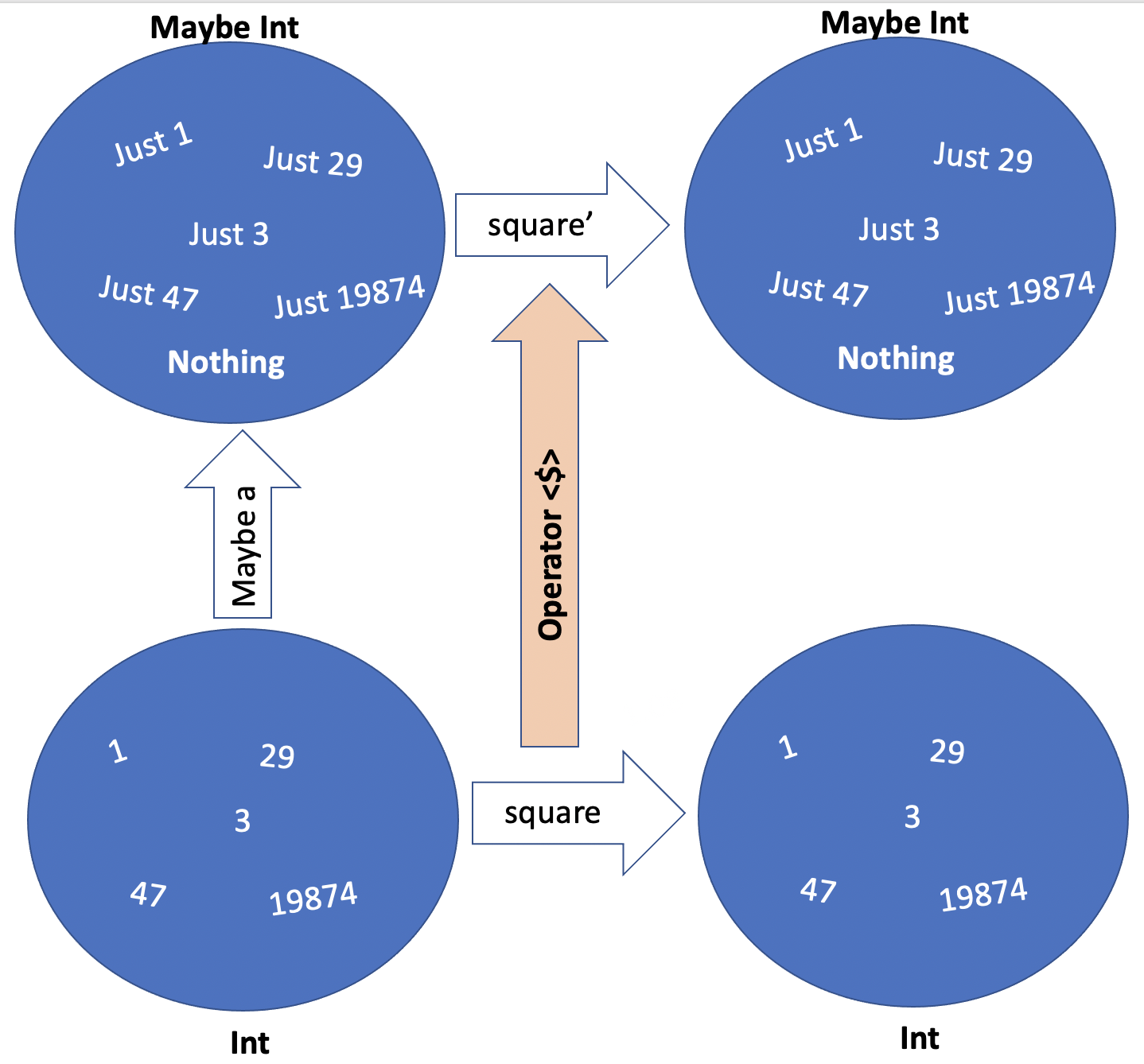
By looking at this attentively and thinking hard, we can easily design operator <$> for Maybe like this (note also operator definition syntax):

1 (<$>) :: (a -> b) -> Maybe a -> Maybe b
2 (<$>) f Nothing = Nothing
3 (<$>) f (Just x) = Just (f x)

It takes a function between some concrete types a and b and turns it into a function between corresponding Maybes. Now, Maybe a is a type function that you should read as Maybe (a:Type) = ... What other type functions do we know by now? Of course it’s a List, or [a]! Can you define operator <$> that would take a function a -> b and turn it into a function between corresponding lists - [a] -> [b]? I know you can. Do it. Do it now.

Good. As they say, one is a coincidence, two is a trend, so why don’t we take it further – what if we had some type function type function f (a : Type) = ... or, in haskell, f :: * -> * (a function that takes a concrete type and creates another concrete type from it) that may have different constructor functions, just like Maybe or List – can we define operator <$> for it? Something like:

1 (<$>) :: (a -> b) -> f a -> f b

We want this operator, just like in case of Maybe and List, to take a function g :: a -> b and turn it into a function that is lifted into our type function f - h :: f a -> f b. Let’s write out full signatures in our pseudocode to make sure we are clear on what means what. Operator <$> takes a function g (x:a) : b (takes a value of type a and returns a value of type b) and turns it into a function h ( x : f(a:Type) ) : f(b:Type) (takes a value of type f a and returns a value of type f b)

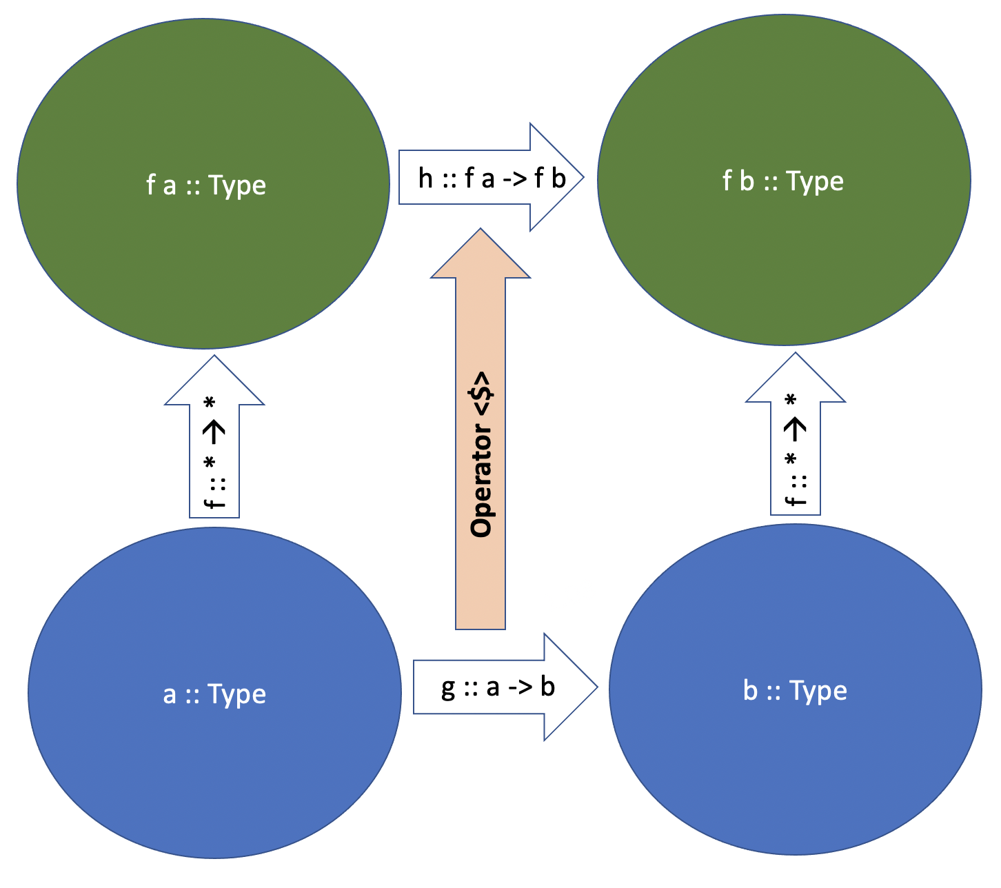
Congratulations, you just invented a Functor. A Functor is merely any type function f :: * -> *, like Maybe a or list [a] that has an operator <$> defined, which “converts” or lifts functions between two concrete types – g :: a -> b – to functions between values of types constructed from a and b with the help of our type function f – h :: f a -> f b. In Haskell, Functor is a typeclass - more on this in a bit in Chapter 3.

Why do we need functors? So that we can write g <$> lst and be sure our “simple” g function works on complicated values constructed with some type function – instead of resorting to verbose boilerplate nested case statements for each new type we define. Ah, yes - if you wrote operator <$> for list above you should have noticed that’s it’s merely the map function. So Functor is our first very useful abstraction. If you define some type function f that takes some concrete type and creates another concrete type from it - similar to Maybe or List - always check if you can turn it into Functor by defining a <$> operator. This will make your code concise, easy to read, breeze to maintain.

Most of the confusion in Haskell stems from the fact that the concepts here are named almost exactly as they are in category theory, which is about the only actively developing area of mathematics nowadays, cutting edge of the most abstract of science. I mean, why not call this an elevator or injector or something less scary than a Functor?! But it is what it is: really really simple elegant concept named so as to confuse us simple folk. However, for those who wish to be more technical, we will have a chapter on light Category Theory intro as well.

Let us open the floodgates!