5 4 Paths and complex shapes
In the previous chapter Basic drawing operations we looked at ways to draw simple shapes. In this chapter we will extend this to look at more complex shapes, with practical examples. We will also take a closer look at paths and sub-paths.
5.1 4.1 Paths
A path is the most general type of shape. It is made up of one or more edges, than can consist of straight lines, arcs, or curves (specifically Bezier curves).
For example:
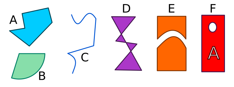
- Path A is created from 6 straight lines.
- Path B consists of 2 straight lines and a circular arc.
- Path C consists of 2 straight lines and 2 Bezier curves.
Each of the paths in the image has its own characteristics, to illustrate the variety of different forms a path can take:
- A and B are simple closed paths, that each enclose a single area. A is a polygon, B is a sector of a circle.
- C is an open path, it is just a set of lines that don’t enclose an area. An open path has two end points that are not joined together.
- D is a self-intersecting path. It is a polygon just like A, but some of its sides cross over, so it encloses several different areas (4 triangular areas in this case).
- E is a disjointed path. It consists of 2 separate closed shapes (each shape is actually a sub-path, which we will explain in the next section).
- F is also a disjointed path, consisting of 3 separate closed shapes, but this time the two small shapes (the ellipse and the letter A) actually cut holes in the main rectangular shape. If you placed this shape on top of an image background, you would be able to see the image through the holes.
As example F shows, paths can be text-shaped (the red shape has a text-shaped hole).
Paths are created implicitly, by calling drawing operations on the Pycairo context. But it is also possible to store the path you have created, as a Path object. This can be very useful sometimes as we will see.
5.2 4.2 Sub-paths
Any path is made up of one or more sub-paths. A sub-path is a set of lines or curves joined end to end – each line starts where the previous one ended. A sub-path therefore creates either a single closed shape, or a single set of sequentially joined lines.
In the picture above, each of the four shapes on the left is an example of a path containing a single sub-path. The two shapes on the right are each examples of single paths that are made up of more than one sub-path:
- The orange shape labelled E is made up of two sub-paths (each of the two closed shapes is a separate sub-path).
- The red shape labelled F is made up of three sub-paths (the rectangle itself is one sub-path, the circular hole is another, the A-shaped hole is another).
Letter shapes are a good, practical example of using sub-paths.
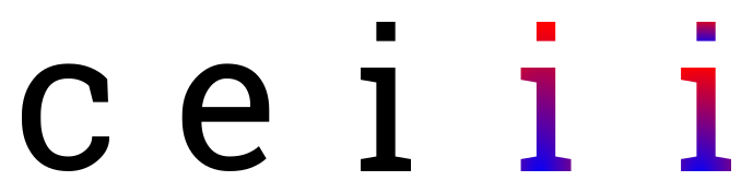
Each of these letters is drawn as a separate path. The letter ‘c’ is a simple closed path. The letter ‘e’ consists of a closed path but it also has a hole in it. This is formed as a sub-path, similar to the example of red shape F, above. Paths with holes aren’t just some fancy effect you might never use, the page you are reading contains hundreds of examples.
The letter ‘i’ is interesting. It consists of two separate shapes (the main character and the dot above it), but of course they are part of the same letter shape. You wouldn’t usually want to show one without the other, and you would always want them to be in the same position relative to each other – if you put the dot underneath the main character, for example, it wouldn’t be a letter ‘i’ any more! So it makes perfect sense to have those two shapes as two sub-paths of the same path.
The second letter ‘i’ shows another advantage of sub-paths. We have filled this letter with a gradient (the colour changes from blue to red, vertically). Since the two shapes are both sub-paths of the same path, the gradient is applied across the entire letter, from the base right to the top of the dot.
The third letter ‘i’ shows how the gradient might look if the two parts of the letter were drawn as completely separate paths. The dot now has its own blue to red gradient, which is probably not the effect you would want.
When we look at text in a later chapter, we will see that often a whole word (or sentence, or paragraph) of text is drawn as a single path with lots of sub-paths (one or more for each letter).
5.2.1 4.2.1 Creating sub-paths
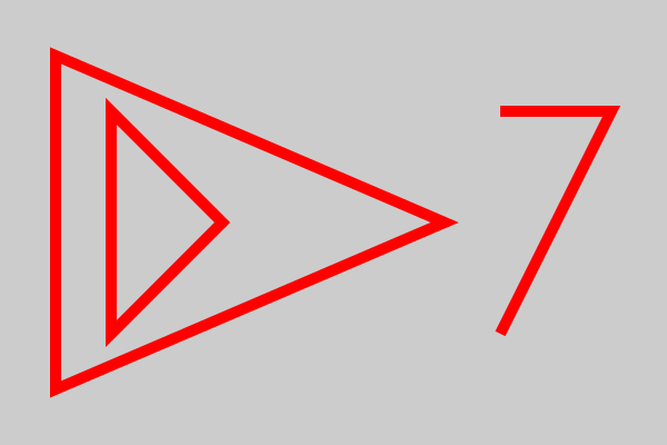
The most common way of creating a new sub-path is the move_to function. Here is some code that creates a path consisting of 3 sub-paths:
#Sub-path 1
ctx.move_to(50, 50)
ctx.line_to(400, 200)
ctx.line_to(50, 350)
ctx.close_path()

#Sub-path 2
ctx.move_to(450, 100)
ctx.line_to(550, 100)
ctx.line_to(450, 300)

#Sub-path 3
ctx.move_to(100, 100)
ctx.line_to(200, 200)
ctx.line_to(100, 300)
ctx.close_path()

ctx.set_source_rgb(1, 0, 0)
ctx.set_line_width(10)
ctx.stroke()
Sub-path 1 is started by the first move_to. It is a closed triangle with corners at (50, 50), (400, 200) and (50, 300). The call to close_path at the end of the definition closes the sub-path (ie it joins the final point to the initial point).
Sub-path 2 is started by the second move_to. It is an open shape with two sides. There is no close_path because the shape is not closed.
Sub-path 3 is started by the third move_to, and creates another closed triangle with corners at (100, 100), (200, 200) and (100, 300).
The final call to stroke draws the entire path (containing 3 sub-paths) and clears the path afterwards. Here is the image created:
You can also create a new sub-path using the context function new_sub_path. This is similar to move_to, but it doesn’t set the current point. It is mainly used with the arc function as described later in this chapter.
The final way to create a new sub-path is the rectangle function. This creates a closed rectangular sub-path, see later in this chapter.
5.3 4.3 Lines
We know how to draw a line between two points (x1, y1) and (x2, y2), like this:
ctx.move_to(x1, y1)
ctx.line_to(x2, y2)
Now we will look at a couple of other examples.
5.3.1 4.3.1 Drawing a line of given length and angle
In this case we will see how to draw a line that:
- Starts from the point
(x1, y1). - Is at an angle
afrom the x-axis. - Has length
r.
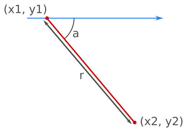
To draw this line, we need to find the position of the second point (x2, y2). We can use trigonometry to do this. We use the line to form a right-angled triangle, with the two short sides aligned with the x-axis and y-axis:
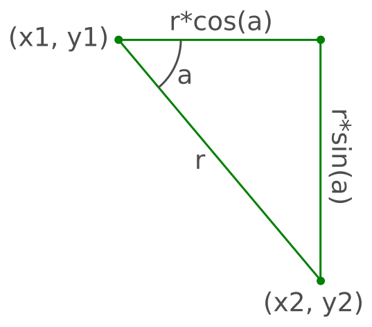
From this diagram we can see that:
x2 = x1 + r*math.cos(a)
y2 = y1 + r*math.sin(a)
So, the code to draw the line of a given length and angle is:
5.3.2 4.3.2 Relative drawing functions
In the example above, the position of (x2, y2) is calculated as an offset from the current point (x1, y1). Its relative position is calculated.
The function rel_line_to allows us to specify the new point relative to the current point. We can simplify our drawing code like this:
ctx.move_to(x1, y1)
ctx.rel_line_to(r*math.cos(a), r*math.sin(a))
There is also a rel_move_to function and a rel_curve_to function, that operate in a similar way.
5.4 4.4 Polygons
In this section we will look at a slightly more complex polygons – a useful arrow shape. This example will illustrate a few techniques than can be used generally to design polygons.
5.4.1 4.4.1 A simple arrow
Here we will see how to draw this arrow:
The size and position of the arrow is defined by its bounding box (x, y, width, height). The shape of the arrow can be adjusted by controlling the tail length a and inset b.
The shape has 7 vertices, which we will number:
We can calculate the position of each vertex:
1. (x, y + b)
2. (x, y + height – b)
3. (x + a, y + height – b)
And so on. To draw the arrow, we just join the points to make a polygon. Here is a function that draws an arrow:
def arrow(ctx, x, y, width, height, a, b):
    ctx.move_to(x, y + b)
    ctx.line_to(x, y + height - b)
    ctx.line_to(x + a, y + height - b)
    ctx.line_to(x + a, y + height)
    ctx.line_to(x + width, y + height/2)
    ctx.line_to(x + a, y)
    ctx.line_to(x + a, y + b)
    ctx.close_path()
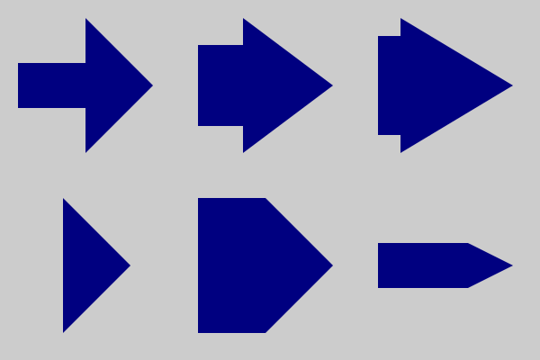
This code is quite versatile, we can create different arrow shapes by varying the size of the bounding box (width and height) and changing a and b. Here are some examples:
ctx.set_source_rgb(0, 0, 0.5)
arrow(ctx, 20, 20, 150, 150, 75, 50)
ctx.fill()
arrow(ctx, 220, 20, 150, 150, 50, 30)
ctx.fill()
arrow(ctx, 420, 20, 150, 150, 25, 20)
ctx.fill()
arrow(ctx, 70, 220, 75, 150, 0, 50)
ctx.fill()
arrow(ctx, 220, 220, 150, 150, 75, 0)
ctx.fill()
arrow(ctx, 420, 270, 150, 50, 100, 0)
ctx.fill()
This is the image the code creates:
5.5 4.5 Arcs
We took a quick look at arcs in an earlier chapter. This time we will look more closely at how angles are interpreted and how arcs connect to other lines and curves.
5.5.1 4.5.1 Arc angle rules
The arc function looks like this:
ctx.arc(x, y, r, a1, a2)
It draws an arc of a circle, centre (x, y) and radius r. The arc starts at angle a1 and ends at angle a2. Here is an example:
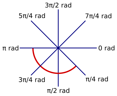
The red arc was drawn with the following call:
ctx.arc(x, y, r, math.pi/4, math.pi)
There are several things to notice this:
- The angle 0 points horizontally to the left, that is in the direction of the x-axis.
- Angles increase as you move clockwise.
- The arc is drawn from the first angle to the second angle in the direction of increasing angles (ie clockwise).
The arc is drawn as follows:
- The start of the arc
a1, i.e.pi/4. - The length of the arc is
a2 – a1, i.e.(pi – pi/4)which is3*pi/4. - Therefore, the arc starts at
pi/4and covers an angle of3*pi/4.
Here is another example:
ctx.arc(x, y, r, 7*math.pi/4, math.pi/4)
In this example, a2 is less than a1. In that case Pycairo adds 2*pi to a2, repeatedly, until the result is greater than a1. In this case we only need to add 2*pi once, giving 9*pi/4. This creates the following arc:
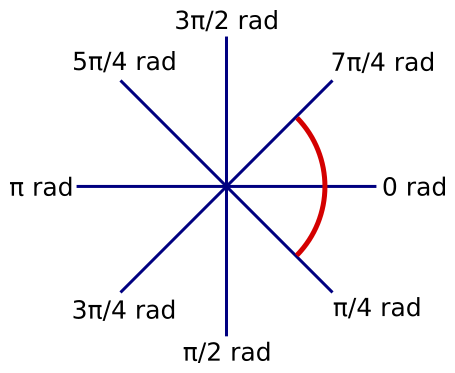
- The start of the arc
a1, i.e.7*pi/4. - The length of the arc is
a2 – a1, i.e.(7*pi/4 – 9*pi/4)which ispi/2. - Therefore, the arc starts at
7*pi/4and covers an angle ofpi/2.
Here are some more examples:
ctx.arc(x, y, r, 0, 0)         # 1
ctx.arc(x, y, r, 0, 2*math.pi) # 2
ctx.arc(x, y, r, 0, 3*math.pi) # 3
Case #1 will draw an arc of length 0. The rule above says that we must add 2*pi to a2 if a2 is less than a1. But in this case the two angles are equal, so a2 is not less than a1. We don’t need to add 2*pi.
Case #2 has an arc angle of 2*pi, which is a full circle. This code draws a complete circle.
Case #3 has an arc angle of 3*pi, which is a one and a half full circles. This code draws a complete circle, but the current point is left at the position determined by the actual final angle of 3*pi.
5.5.2 4.5.2 Arcs and the current point
When we use the line_to function, we only specify an end point. The function draws a line from the current point to the supplied end point.
arc is slightly different. By specifying the start and end angles, it implicitly defines the start and end points of the curve it draws. So how does the current point fit in?
There are two cases:
- If you create an arc when there is no current point defined, the arc starts at
a1as in the examples so far. - If you create an arc when there is already a current point defined, a straight line is created from the current point to
a1, then the arc is drawn as normal.
In both cases, the current point is set to the end of the arc afterwards. We will see some examples of this, next.
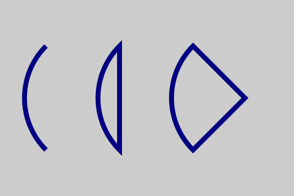
5.5.3 4.5.3 Sectors and segments
The image below shows an arc, a segment and a sector. To illustrate how arcs interact with the current point, all three shapes are added as sub-paths within a single path.
Here is the drawing code:
ctx.set_line_width(10)
ctx.set_source_rgb(0, 0, 0.5)

# Arc
ctx.arc(200, 200, 150, 3*math.pi/4, 5*math.pi/4)

# Segment
ctx.new_sub_path()
ctx.arc(350, 200, 150, 3*math.pi/4, 5*math.pi/4)
ctx.close_path()

# Sector
ctx.move_to(500, 200)
ctx.arc(500, 200, 150, 3*math.pi/4, 5*math.pi/4)
ctx.close_path()

ctx.stroke()
The first (left hand) figure is just an arc. Since we are at the start of a new path, there is no current point, so we can just draw the arc as a standalone shape.
The second (centre) figure is a segment – that is, an arc with its ends joined. However, at this point we already have a current point defined – it is set to the end of the previous arc. If we just draw an other arc, we will get an unwanted line from the old arc to the new one.
We can avoid this by calling new_sub_path. This function starts a new sub-path but without defining a current point. It is like calling move_to except it leaves the current point undefined.
We then draw the arc, followed by a call to close_path. The call to close_path draws a line from the current point (the end of the arc) right back to the first point in the current sub-path (the start of the arc). This creates the segment shape.
The final shape, on the right, is a sector – a pie wedge. We draw this shape like this:
-
move_tothe centre of the arc. This starts a new sub-path with a defined current point. - Add the arc. This automatically adds a line from the current point at the centre of the arc to the start point of the arc, and then adds the arc itself.
- Call
close_path. This adds another line from the end of the arc to the start of the sub-path (ie the centre of the arc).
Notice that we have not explicitly drawn either of the straight lines! In the next example we will draw a roundrect shape without drawing any straight lines at all.
5.5.4 4.5.4 Roundrect
A roundrect is a rectangle with rounded corners:
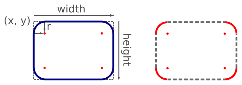
It is defined by its position (x, y), width, height, and the radius r of the rounded corners. As the right-hand side of the diagram shows, a roundrect is made up of four quarter circles of radius r, with fours straight lines between them.
The most important points for drawing a roundrect are the centres of the corner circles. These are inset from the corners of the enclosing rectangle by an amount r. Starting from the top left corner and working clockwise, these centre points are:
- (x + r, y + r)
- (x+width-r, y+r)
- (x+width-r, y+height-r)
- (x+r, y+height-r)
The diagram below shows how we create the roundrect. The red solid lines show the arcs that we explicitly draw, the grey dashed lines show the connecting lines that Pycairo draws automatically:
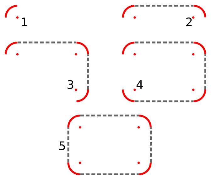
- We draw the first quarter circle arc.
- We draw the second quarter circle arc. Pycairo automatically draws a line from the end of the previous arc to start of the new arc.
- We draw the third quarter circle arc, and again Pycairo draws a line from the end of the previous arc to the start of the new one.to start of the new arc.
- We draw the fourth quarter circle arc, and again Pycairo draws the extra line.
- Finally we close the path, so Pycairo adds a line from the end of the last arc to the start of the first arc, completing the shape.
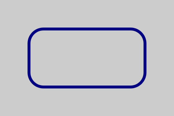
Here is the code to do this:
def roundrect(ctx, x, y, width, height, r):
    ctx.arc(x+r, y+r, r, math.pi, 3*math.pi/2)
    ctx.arc(x+width-r, y+r, r, 3*math.pi/2, 0)
    ctx.arc(x+width-r, y+height-r, r, 0, math.pi/2)
    ctx.arc(x+r, y+height-r, r, math.pi/2, math.pi)
    ctx.close_path()

ctx.set_line_width(10)
ctx.set_source_rgb(0, 0, 0.5)
roundrect(ctx, 100, 100, 400, 200, 50)
ctx.stroke()
Here is the final result:
5.5.5 4.5.5 arc-negative
The arc_negative function is exactly the same as the arc function, except that the arc goes in the opposite direction. This code illustrates the difference:
ctx.set_line_width(10)
ctx.set_source_rgb(0, 0, 0.5)
ctx.arc(150, 200, 100, 3*math.pi/4, 5*math.pi/4)
ctx.stroke()
ctx.arc_negative(400, 200, 100, 3*math.pi/4, 5*math.pi/4)
ctx.stroke()
The arc function draws an arc from angle 3*math.pi/4 to angle 5*math.pi/4 in the direction of increasing angles (clockwise by default). The arc_negative function draws an arc from angle 3*math.pi/4 to angle 5*math.pi/4 in the opposite direction. In the image, arc is on the left and arc_negative is on the right (the dashed circle illustrates the whole circle in each case):

You can do the same thing by swapping the start and end angles in the standard arc function, but arc_negative can be more intuitive in some cases.
5.6 4.6 Bezier curves
A Bezier curve is a commonly used curve in vector graphics. It is versatile, efficient to work with, and has many useful properties.
A cubic Bezier curve is the most often used type, and is actually the only one supported by Pycairo. It is defined by four points A, B, C, D:
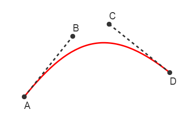
The points A and D are called the anchors, and are always located at the two ends of the curve. The points B and C are called the handles, and control the basic shape of the curve. The curve will generally follow the form of the open shape ABCD.
Pycairo defines a Bezier curve with the function curve_to:
ctx.move_to(ax, ay)
ctx.curve_to(bx, by, cx, cy, dx, dy)
ctx.set_source_rgb(1, 0, 0)
ctx.set_line_width(2)
ctx.stroke()
In the code, point A is represented by coordinates (ax, ay), point B by (bx, by) etc.
The curve uses move_to to set the current point as the point A. The curve_to function treats the current point as point A, and accepts the coordinates of points B, C, D as parameters.
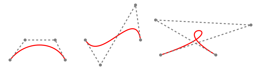
5.6.1 4.6.1 Common forms
In you keep the end points A and D fixed, you can create a variety of different shapes by moving the handles B and C around. There are 3 basic forms:
- A simple curve.
- An S shaped curve.
- A looped curve.
These are illustrated here.:
The curve always fits entirely within the convex hull of the points A, B, C, D:
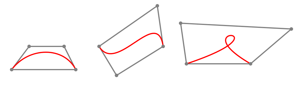
Here is a larger selection of possible shapes:
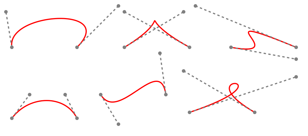
The best way to explore Bezier curves is probably to use a vector graphics editor. Inkscape is an excellent, free product that runs on Windows, Linux and Mac. You can experiment with shapes and read off the positions of the nodes when you have a shape you like.
5.6.2 4.6.2 Splines
Sometimes you might want to draw a more complex curved shape. For example in a 2D computer game you might have characters, spaceships, clouds, etc. These can be draw by joining several Bezier curves together. A composite curve, constructed from more than one base curve joined end to end, is called a spline. Bezier curves are an excellent choice for making splines. Not only are they easily adjustable to match a shape locally, but they can also joined smoothly.
It is quite easy to join two or more Bezier curves. We just need to define the curves so that they have a shared anchor point.
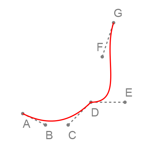
The diagram below shows two Bezier curves that are joined. The first curve has anchor points A and D, with handles B and C. The second curve has anchor points D and G, with handles E and F. Since the curves both have point D as an anchor, they are joined at that point.
The code to draw two joined Bezier curves looks like this:
ctx.move_to(ax, ay)
ctx.curve_to(bx, by, cx, cy, dx, dy)
ctx.curve_to(ex, ey, fx, fy, gx, gy)
Here is how it works:
-
move_tosets the current point to point A. -
curve_todraws a curve from the current point A to the point D, using B and C as handles. - After executing
curve_tothe current point is set to D - The second
curve_todraws a curve from the current point D to the point G, using E and F as handles.
5.6.3 4.6.3 Smooth curves
In the diagram above, you will notice that the two Bezier curves form a corner where they connect. There is nothing wrong with that, it is sometimes what you want to create a particular shape.
Other times you might want two Bezier curves to join more smoothly, so it looks like a single curve, as shown below:
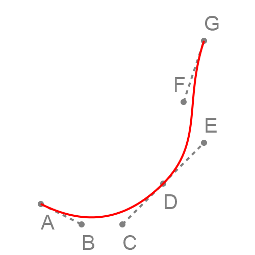
It is fairly easy to do this. The slope of a Bezier curve at its end point is equal to the slope of the line from the handle. That is:
- For the first curve, the slope of the curve at point D is the same as the slope of the line between C and D.
- For the second curve, the slope of the curve at point D is the same as the slope of the line between D and E.
This means that if the points C, D and E are all in a straight line (as they are in the example), the two curves will have the same slope where they meet, which avoids a corner.
In other words, to obtain a smooth join, make sure the handles of the two curves line up.
Another thing to know is that the second derivative of the curve at its end point is determined by the length of the line to the handle. The second derivative means the rate of change of the slope, or very loosely speaking how curved the Bezier curve is near its end point. If the two curves have the same slope and curvature, the join will be even more smooth.
So, to get the smoothest result when joining two curves, ensure that:
- The handles C and E, and the anchor D are in a straight line.
- The distance from C to D is the same as the distance from D to E .
5.7 4.7 Function curves
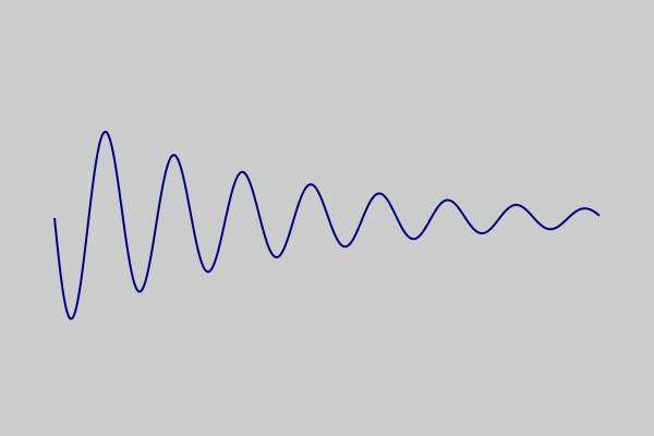
Sometimes you might want to draw a curve based on a mathematical function. Here is an example of a function y = f(x):
y = math.sin(10*x)*math.exp(-x/2)
This function is a decaying sine wave. It represents simple damped oscillation - for example, the sound created if you pluck a guitar string, that starts off loud and gradually fades away. Don’t worry too much about the details of the function, we are mainly using it because it looks quite nice. This is a graph of the function created using Pycairo:
How is that done? Well, it is actually quite simple. We choose a series of value of x, and calculate f(x) for each value. This gives us a set of points that lie on the curve:
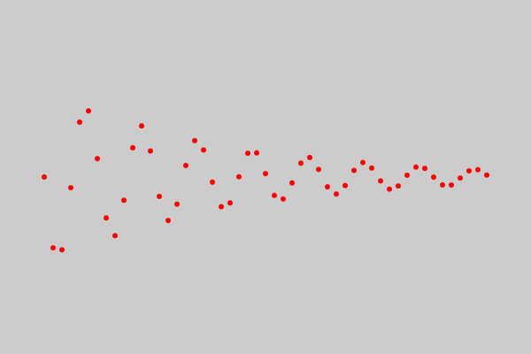
We then join this points with straight lines. In other words, we create a polyline from all the points.
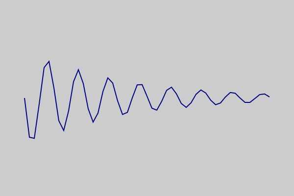
Now this looks pretty lumpy at the moment, you can clearly see the individual lines. That is deliberate, to show what is going on. The trick is to calculate more points that are closer together, then they look like a smooth curve.
Now we can move on to the actual code that creates the function curve above. Here is how we calculate the points:
x = 0
points = []
while x < 5:
    y = math.sin(10*x)*math.exp(-x/2)
    points.append((x*100 + 50, y*100 + 200))
    x += 0.01
The while loop iterates over values of x from 0.0 to (almost) 5.0 in steps of 0.01. The step value is very important, it determines the gap between the calculated points, which controls how smooth the curve is. You need to experiment a bit, if the gap is too big the curve won’t be smooth, but if it is too small you will be calculating more points than you really need to.
For each x value, we calculate a y value using our function (the decaying sine wave function).
The result to of this is a set of (x, y) values that we want to plot. But there is a slight problem. Our x values are in the range 0.0 to 5.0. Our y values are in the range -1.0 to +1.0. If we plot those points on a canvas that is 600 units by 400 units, we will end up with a tiny graph stuck in the top corner!
We need to scale and translate our x and y values to create a set of points that have sensible canvas locations. Here is what we do:
- For
xvalues we multiply by 100 and add 50. Soxvalues in the range 0.0 to 5.0 create canvas values in the range 50 to 550 - ideal for a canvas that is 600 units wide. - For
yvalues we multiply by 100 and add 200. Soyvalues in the range -1.0 to +1.0 create canvas values in the range 100 to 300 - also ideal for a canvas that is 400 units high.
We add these scaled points to the points list, as (x, y) tuples.
Plotting the points is now quite easy:
ctx.move_to(*points[0])
for p in points[1:]:
    ctx.line_to(*p)

ctx.set_line_width(2)
ctx.set_source_rgb(0, 0, 0.5)
ctx.stroke()
We move_to the location of points[0], and then call line_to on the rest of the points in the list to create a polyline. We then stroke the polyline.
5.8 4.8 Rectangle
We met the rectangle function in the chapter Basic drawing operations. There isn’t a lot more to say about it really, it draws a rectangle!
The call rectangle(x, y, width, height) is roughly equivalent to this code:
ctx.move_to(x, y)
ctx.line_to(x + width, y)
ctx.line_to(x + width, y + height)
ctx.line_to(x, y + height)
ctx.close_path()
It creates a new sub-path with move_to and closes the path when it has finished.