4 3 Basic drawing operations

In vector graphics, we don’t directly paint individual pixels. Instead, we define shapes and tell Pycairo how we want them to be filled or outlined.

Our completed image can be stored as a vector image (such as SVG) or it can be converted into a raster format such as PNG. In most of the examples in this chapter we will create PNG files, but we will also see how to create other types of output.

Drawing shapes is a very important aspect of Pycairo programming, so we have devoted two chapters to the topic. In this chapter we will learn about the basic shape functions and how to use them to create simple images in Pycairo. In a later chapter we will revisit this and look at practical examples of creating more complex shapes.

4.1 3.1 Creating an image with Pycairo

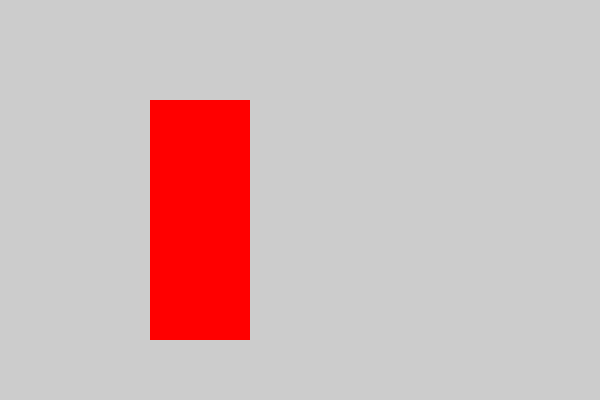
We will start by creating a very simple PNG image, containing just a single rectangle. Here is the code:

import cairo

# Set up pycairo
surface = cairo.ImageSurface(cairo.FORMAT_RGB24, 600, 400)
ctx = cairo.Context(surface)
ctx.set_source_rgb(0.8, 0.8, 0.8)
ctx.paint()

# Draw the image
ctx.rectangle(150, 100, 100, 240)
ctx.set_source_rgb(1, 0, 0)
ctx.fill()

# Save the result
surface.write_to_png('rectangle.png')

Here is image this creates:

We will go through this code, step by step, to gain a better understanding of how Pycairo creates images.

4.1.1 3.1.1 Setting up Pycairo

You will need to have Python and Pycairo installed on your system (see the chapter About Pycairo). As with any Python module, you must import it before you can use it:

import cairo

Next, we must create a surface. A surface is the object where you create your image. You can think of it a bit like an artist’s canvas:

surface = cairo.ImageSurface(cairo.FORMAT_RGB24, 600, 400)

When we create the surface, we are also deciding what sort of output we are going to produce:

• An ImageSurface will create a PNG image as output. There are other types of surface that create different output formats, for example SVG or PDF.
• We set the format to FORMAT_RGB24, which is a normal RGB image.
• We set the output image size to 600 by 400 pixels.

The next step is to create a context. A context is the thing we use to draw on the surface. You could think of it as being analogous to a pen that draws on the surface, but this is quite a loose analogy. Here is how we create a context:

ctx = cairo.Context(surface)

Finally, we will fill the entire surface with a light grey colour, using the paint function:

ctx.set_source_rgb(0.8, 0.8, 0.8)
ctx.paint()

The Context function set_source_rgb is used to set a colour. The colour is determined by 3 values that control the amount of red, green and blue in the colour. Values of 0 mean none of that colour is present, values of 1 means that the colour is as bright as possible. Setting the colour to (0.8, 0.8, 0.8) means that the red, green and blue values are each set to 80% of their maximum, which gives a light grey colour. See the chapter Colour for more details.

The paint function fills the entire surface with the previously selected colour. This is why the image (above) has a light grey background.

4.1.2 3.1.2 Drawing the image

This is the code that draws the red rectangle:

# Draw the image
ctx.rectangle(150, 100, 100, 240)
ctx.set_source_rgb(1, 0, 0)
ctx.fill()

Drawing in Pycairo is a two-step process. First, we define a path. A path is an abstract description of what we intend to draw. The second stage is to actually draw the shape described by the path.

The rectangle function adds a rectangle shape to the path. It doesn’t draw a rectangle, it just adds it to the plan of what we are intending to draw. The function has the following definition:

rectangle(x, y, width, height)

It specifies a rectangle placed at position (x, y) with the given width and height. Our code will place a rectangle at position (150, 100), with a width of 100 and a height of 240. We will explain how coordinates work in a little while.

Next, we set our colour with set_source_rgb, this time to (1, 0, 0), which is 100% red with no green or blue – in other words, bright red.

Finally, we call fill. This function looks at the path we have defined and fills it with the colour we previously selected. The fill function is what actually draws the shape, in this case a rectangle.

4.1.3 3.1.3 Saving the PNG file

When we have finished drawing, we can save the image as a PNG file:

# Save the result
surface.write_to_png('rectangle.png')

This saves the image to the file rectangle.png in the current folder (usually wherever the Python source file is). Of course, you could add a full file path rather than just a filename if you wanted to write the file to a specific folder.

Notice that write_to_png is a function of the Surface object. This makes sense if you think about it, the surface is the object that owns the image.

Now that we know how to draw a simple image, we will learn a bit more about the way Pycairo defines the position and size of objects (ie the coordinate system), and how to draw a variety of other simple shapes.

For the rest of this chapter, all the examples will use the same basic code to draw a 600 by 400 pixel image. For brevity, we will only show the code that belongs in the Draw the image section of the code.

4.2 3.2 Coordinate system

By default, Pycairo uses a simple coordinate system based on the size of the output image you are creating (specified by the cairo.ImageSurface call). In the previous example, the image is 600 by 400 pixels in size, so the coordinate space is also 600 by 400 units:

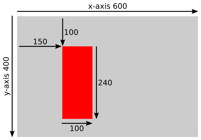
Pycairo coordinates have the origin at the top left of the page, as do many other computer graphics libraries. This is different to the convention used in mathematics, where the origin is usually at the bottom left of the page.

If we look again at the code that defines the red rectangle:

ctx.rectangle(150, 100, 100, 240)

The rectangle is positioned at point (150, 100). This means that the top left corner of the rectangle is positioned 150 pixels to the right and 100 pixels down from the top left corner of the image. The rectangle itself is 100 pixels wide and 240 pixels high.

4.3 3.3 Rectangles

In this next example we will draw two rectangles and a square. Here is the code:

ctx.rectangle(150, 100, 100, 240)
ctx.set_source_rgb(1, 0, 0)
ctx.fill()

ctx.rectangle(300, 100, 100, 240)
ctx.set_source_rgb(0, 1, 0)
ctx.fill()

ctx.rectangle(350, 170, 200, 200)
ctx.set_source_rgb(0, 0, 1)
ctx.fill()

This code is similar to the previous example code, but we have extended it to draw 3 rectangles. In each case, we set the position and size (different for each rectangle), select the colour (a red, a green and a blue rectangle), and call fill to draw the rectangle.

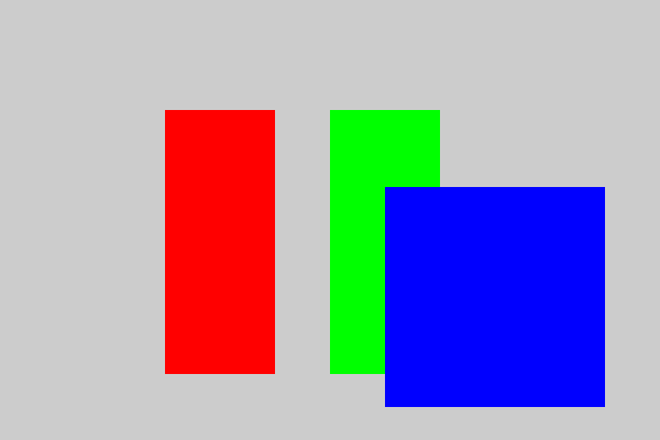
One thing to notice is that the blue square partially overlaps the green rectangle. This is not uncommon in computer graphics. Pycairo handles this in a consistent way. Each new object is painted over the top of any existing objects. The green rectangle is painted first, then the blue square is painted on top of it.

4.4 3.4 Fill and stroke

So far, we have drawn filled rectangles. Sometimes you might just want to draw the outline of a shape. This is called stroking (as in a stroke of the pen).

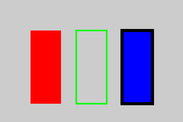
You can also fill and stroke a shape, usually with different colours. Here is an example of each case. The red shape on the left is filled, the green shape in the middle is stroked, the blue shape on the right is filled and stroked (in black).

Here is the code to draw the red filled shape. This is the same as the previous example:

# Fill
ctx.rectangle(100, 100, 100, 240)
ctx.set_source_rgb(1, 0, 0)
ctx.fill()

Here is the code to draw the green stroked shape:

# Stroke
ctx.rectangle(250, 100, 100, 240)
ctx.set_source_rgb(0, 1, 0)
ctx.set_line_width(5)
ctx.stroke()

We use the rectangle function, as normal, then use set_source_rgb to set the colour of the outline. There is then an extra step – we call set_line_width to choose how wide the outline should be. Line width is measured in the units of the coordinate system. The whole rectangle is 100 units wide, so a 5 unit outline gives a moderately thick outline. Calling the stroke function then draws the outline of the rectangle, using the required colour and thickness.

And here is how to draw the blue filled and stroked shape:

# Fill and stroke
ctx.rectangle(400, 100, 100, 240)
ctx.set_source_rgb(0, 0, 1)
ctx.fill_preserve()
ctx.set_source_rgb(0, 0, 0)
ctx.set_line_width(10)
ctx.stroke()

This is similar to the previous examples. We define the rectangle shape. Then we set the blue colour and fill the shape. Then we set the black colour, set the line width, and stroke the shape.

There is just one little wrinkle. We said earlier that the rectangle function adds a rectangle shape to the path, ready to be drawn. There is something else we need to know – the fill and stroke functions not only draw the path, they also clear the path afterwards.

This is usually what we want. Normally we define a path, then either fill it or stroke it, and then it the path has been automatically cleared, so we can carry on and draw the next shape.

However, if you want to fill and stroke a shape, you have an obvious problem. You create the path and fill it, but then the path is deleted so you can stroke it. The fill_preserve function does the same job as fill, but it doesn’t clear the path. We can then use stroke to outline the same rectangle. We will look at this is a bit more detail is the chapter Paths and complex shapes.

4.5 3.5 Lines

So far, we have used rectangles to illustrate drawing in Pycairo. That is a good place to start because the rectangle function is a very convenient way to create a shape.

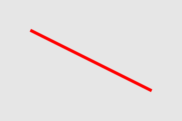
Generally, though, if you need to create any other type of shape, you have to construct it from separate lines and curves. In this section we will see how to draw a simple straight line. Here is the code we use to do this:

ctx.move_to(100, 100)
ctx.line_to(500, 300)
ctx.set_source_rgb(1, 0, 0)
ctx.set_line_width(10)
ctx.stroke()

And here is the image it creates:

Pycairo uses the idea of a current point when drawing shapes. This makes it easy to create common shapes, such as polygons, that are formed from lines or curves joined end-to-end.

Here is how it works when we draw a line (in the code above):

• Initially the path is empty and the current point is undefined.
• The move_to function sets the current point to (100, 100).
• The line_to function adds a line to the path from the current point to the specified point (500, 300). It also sets the current point to the new value (500, 300).

At this point, the path describes a line from (100, 100) to (500, 300). We then draw this line by setting the colour, setting the line width, and calling stroke. We can’t fill a line, of course, because unlike a rectangle, a line doesn’t enclose an area of the page.

4.6 3.6 Polygons

A polygon is closed shape composed of straight lines. Here is how we draw a simple polygon with 4 sides:

ctx.move_to(50, 100)  # A
ctx.line_to(200, 50)  # B
ctx.line_to(250, 300) # C
ctx.line_to(100, 200) # D
ctx.close_path()
ctx.set_source_rgb(1, 0, 0)
ctx.set_line_width(10)
ctx.stroke()

This draws the shape below:

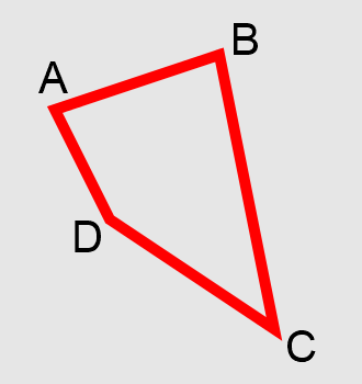
Here is the sequence of events:

• Initially, the path is empty and the current point is undefined.
• move_to sets the current point to A.
• line_to adds a line to the path, from the current point A to the point B. It also sets the current point to the new value B.
• line_to adds another line from B to C, and sets the current point C.
• line_to adds another line from C to D, and sets the current point D.
• close_path completes the closed shape. It adds a line from the current point D back to the first point in the path, which was A.

As before, we set the colour and line width, then stroke the path to draw the polygon.

An important point here is that close_path actually joins point D to point A. It makes the corner look like a proper joined corner. Don’t be tempted to use another line_to to join point D to point A. It will draw a line, but it won’t create a proper corner at A. This is the effect – the lines at corner A don’t join correctly, making it different to the other corners:

4.7 3.7 Open and closed shapes

We can also create open shapes – a set of lines that join end-to-end but don’t join start to end. This is called an open-polygon, or sometimes a polyline. Here is an example:

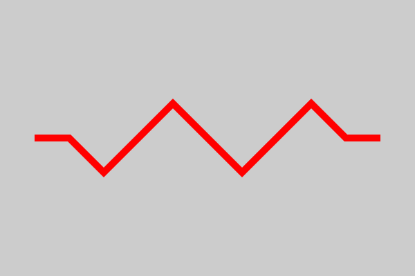
ctx.move_to(50, 200)
ctx.line_to(100, 200)
ctx.line_to(150, 250)
ctx.line_to(250, 150)
ctx.line_to(350, 250)
ctx.line_to(450, 150)
ctx.line_to(500, 200)
ctx.line_to(550, 200)
ctx.set_source_rgb(1, 0, 0)
ctx.set_line_width(10)
ctx.stroke()

We create an open shape in the same way we create a closed shape, except we don’t call close_path at the end. Open shapes can be used for decorative dividers, symbols, arrows and many other applications.

4.8 3.8 Arcs

An arc is a part the circumference of a circle. The arc function is called like this:

ctx.arc(cx, cy, r, a1, a2)

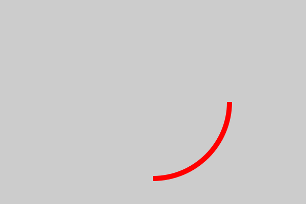
This code will create an arc like this:

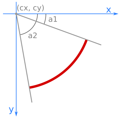
The arc is part of a circle, radius r, centred at the point (cx, cy). The arc starts at angle a1 and ends at angle a2. Angles are measured from the x-axis, and by default increase as you move clockwise.

Here is an example of the code to draw an arc:

ctx.arc(300, 200, 150, 0, math.pi/2)
ctx.set_source_rgb(1, 0, 0)
ctx.set_line_width(10)
ctx.stroke()

Angles in Python, as in most computer languages, are measured in radians rather than degrees. pi radians is exactly 180 degrees. That makes 1 radian equal to approximately 57.3 degrees.

For more information, see the Reference chapter at the end of the book.

The code above draws an arc of a circle, centre (300, 200) – the middle of the image. The circle radius is 150, and the arc goes from angle 0 to angle pi/2 radians, which is a quarter of a turn. The image looks like this:

4.9 3.9 Circles

There is no function for drawing a circle. Instead, you can just use the arc function again. An arc from 0 to 2*pi radians (which is equivalent to a full circle, 360 degrees) draws a complete circle.

Here is how to draw a circle, centre (cx, cy) and radius r:

ctx.arc(cx, cy, r, 0, 2*math.pi)

4.10 3.10 Bezier curves

A Bezier curve is a versatile curve that can be used to create many different shapes. It is based on four points. The anchors, A and D are the end points of the curve. The control points B and C control the route the curve takes between the anchors.

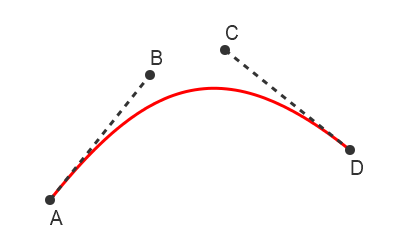
We will cover the properties of this curve is a later chapter, but for now we will just take a quick look at how it works. You might also try experimenting with a drawing package such as Inkscape, which allows you to create Bezier curves and move the 4 points around to try different curves.

Here is the code to draw a single Bezier curve:

ctx.move_to(100, 200)
ctx.curve_to(200, 100, 400, 300, 500, 200)
ctx.set_source_rgb(1, 0, 0)
ctx.set_line_width(10)
ctx.stroke()

Here is the curve it produces:

In the code, move_to sets the current point, in the usual way.

The curve_to function accepts six parameters. It treats the current point as the first anchor A. The six parameters represent the x, y values of the points B, C and D.

After calling curve_to, the current point is set to the location of D, which is the end of the curve.

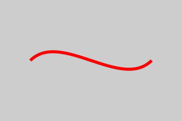
You can also join curves and lines together, to form polycurves. Here we join a curve, a line, and another curve, then close the path (creating another line) to form a shape:

ctx.move_to(100, 100)
ctx.curve_to(200, 0, 400, 200, 500, 100)
ctx.line_to(500, 300)
ctx.curve_to(400, 400, 200, 200, 100, 300)
ctx.close_path()
ctx.set_source_rgb(1, 0, 0)
ctx.set_line_width(10)
ctx.stroke()

Here is the result:

4.11 3.11 Line styles

We will finish this chapter with a look at various ways you can change the appearance of stroked lines. These techniques apply to all stroked lines – single lines, polygons, arcs and Bezier curves.

You might find that you usually just use the defaults, but it is useful to know that other options exist.

4.11.1 3.11.1 Line caps

The line cap value affects how the ends of the lines are drawn. There are three options:

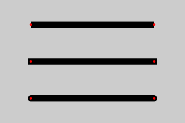
Here is the code to draw these lines:

ctx.set_source_rgb(0, 0, 0)
ctx.set_line_width(20)

ctx.move_to(100, 80)
ctx.line_to(500, 80)
ctx.set_line_cap(cairo.LINE_CAP_BUTT)
ctx.stroke()

ctx.move_to(100, 200)
ctx.line_to(500, 200)
ctx.set_line_cap(cairo.LINE_CAP_SQUARE)
ctx.stroke()

ctx.move_to(100, 320)
ctx.line_to(500, 320)
ctx.set_line_cap(cairo.LINE_CAP_ROUND)
ctx.stroke()

The lines are drawn in the normal way, except that we make an extra call to set_line_cap to set the line cap style for each line.

For illustration, red dots have been added to mark the exact positions of the points passed into the line_to and move_to functions.

The top option is LINE_CAP_BUTT. This is the default if you don’t call set_line_cap at all. The line starts and ends exactly on the points specified, and the ends are squared off. This is useful if you want to ensure that your lines are exactly the right length.

The middle option is LINE_CAP_SQUARE. In this case, the line ends are squared off, but they extend slightly beyond the exact points. In fact, they extend by exactly half of the line width.

The bottom option is LINE_CAP_ROUND. In this case, the line ends are semi-circles, that extend beyond the exact points. The radius of the semi-circle is exactly half the line width.

The choice is largely dependent the visual effect you are wishing to achieve. The line cap style also affects line dashes. You might also prefer to match it with the line join style.

4.11.2 3.11.2 Line joins

You can also control how lines join. Here are the three possible styles:

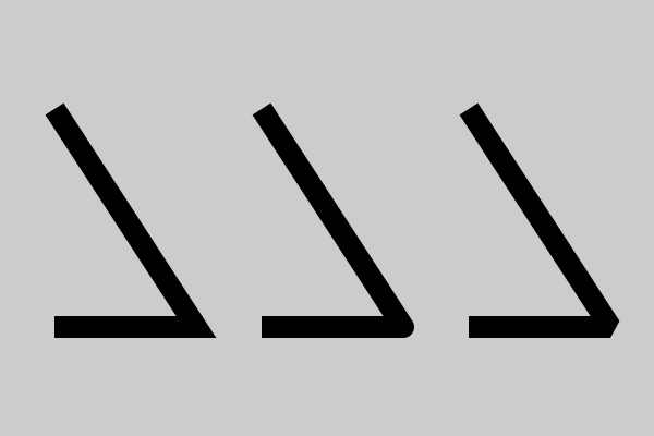
Here is the code to draw these examples:

ctx.set_source_rgb(0, 0, 0)
ctx.set_line_width(20)

ctx.move_to(50, 100)
ctx.line_to(180, 300)
ctx.line_to(50, 300)
ctx.set_line_join(cairo.LINE_JOIN_MITER)
ctx.stroke()

ctx.move_to(240, 100)
ctx.line_to(370, 300)
ctx.line_to(240, 300)
ctx.set_line_join(cairo.LINE_JOIN_ROUND)
ctx.stroke()

ctx.move_to(430, 100)
ctx.line_to(560, 300)
ctx.line_to(430, 300)
ctx.set_line_join(cairo.LINE_JOIN_BEVEL)
ctx.stroke()

We use the set_line_join function to set the style.

The example on the left is LINE_JOIN_MITER. This is the default if you don’t call set_line_join at all. This style creates a pointed corner, similar to a mitre joint used in carpentry.

The middle example is LINE_JOIN_ROUND. This rounds off the point at the corner.

Finally, on the right is LINE_JOIN_BEVEL. This removes the point at the corner with a straight cut.

Notice that these effects only occur where lines actually join, that is:

• The lines are linked by chained calls to line_to, curve_to or arc (similar to the polygons and polycurves we drew earlier).
• The lines is created by close_path, which joins the end point back to the start point in a closed shape.

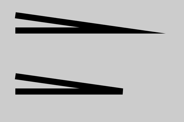
4.11.3 3.11.3 Mitre limit

At this point we will briefly mention the mitre limit. One unfortunate side effect of the mitre join is that at very narrow angles, the length of the mitre point can get stupidly long. In fact, as the angle gets closer to zero, the spike gets longer and longer, without limit!

This isn’t a bug, it is just how mitres work. But it can be quite undesirable, because the spike can start encroaching into parts of the page where it isn’t really wanted.

To avoid this, Pycairo has a mitre limit. If the angle is less than 11 degrees, it automatically uses bevel mode instead of mitre mode. Here is an example, the top join has mitre limit disabled, the bottom one has mitre limit enabled:

You don’t usually need to worry about the mitre limit, it is enabled automatically and in generally a good thing to have. If you really need to change it, you can use the function:

ctx.set_miter_limit(limit)

The limit value determines when the mitre limit applies. In general, if you want the mitre limit to apply at angle a or below, use the following limit value:

limit = 1/math.sin(a/2)

Here are some examples:

• Limit value 1.414 (the square root of 2) applies a mitre limit at 90 degrees or less
• Limit value 2 applies a mitre limit at 60 degrees or less
• Limit value 10 (the default) applies a mitre limit at 11 degrees or less

4.11.4 3.11.4 Dashed lines

Dashed lines are very useful in diagrams and charts. They provide a familiar and intuitive way to distinguish different types of information. For example, if you wanted to add an annotation to a graph, you might enclose it in a box with a dashed outline to indicate that it is additional information, not part of the graph itself.

Dashed lines can also be used purely for decoration.

Of course, drawing a dashed line could potentially be quite complicated, if you needed to draw each dash separately. Fortunately, Pycairo can create a variety of dashed automatically. All you need to do is define the dash pattern, using the set_dash function, like this:

ctx.set_source_rgb(0, 0, 0)
ctx.set_line_width(5)

ctx.move_to(100, 50) #1
ctx.line_to(500, 50)
ctx.set_dash([20])
ctx.stroke() 

ctx.move_to(100, 100) #2
ctx.line_to(500, 100)
ctx.set_dash([20, 10])
ctx.stroke()

ctx.move_to(100, 150) #3
ctx.line_to(500, 150)
ctx.set_dash([20, 5, 5, 5])
ctx.stroke()

ctx.move_to(100, 200) #4
ctx.line_to(500, 200)
ctx.set_dash([5, 5, 10])
ctx.stroke()

ctx.set_line_width(10)
ctx.set_line_cap(cairo.LINE_CAP_ROUND)

ctx.move_to(100, 250) #5
ctx.line_to(500, 250)
ctx.set_dash([10, 20])
ctx.stroke()

ctx.move_to(100, 300) #6
ctx.line_to(500, 300)
ctx.set_dash([0, 20])
ctx.stroke()

This code draws six lines, with different dash patterns. The first four are 5 units wide and use the default butt line cap. The last two are 10 units wide and use the round line cap. They all illustrate different dash patterns:

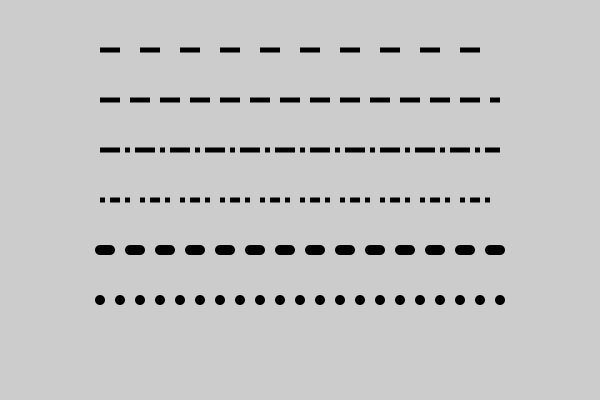
The dash pattern is specified by a list of values that control a repeating sequence of on/off lengths. The lengths are measured in the same units as the line width.

1. The top line is drawn with the pattern [20]. The list is repeated indefinitely to give a sequence 20, 20, 20, 20 … This results in pattern of a 20 unit dash, 20 unit gap, 20 unit dash, 20 unit gap and so on. For brevity we will call this 20 on, 20 off, 20 on, 20 off … It is an evenly spaced line of dashes and gaps.
2. The next line has the pattern [20, 10]. This gives a pattern 20 on, 10 off, 20 on, 10 off … This is similar to the previous pattern but the gaps are shorter than the dashes.
3. This has a pattern [20, 5, 5, 5]. This gives a 20 on, 5 off, 5 on, 5 off … It is a more complex pattern. The gaps are always 5, but the dashes alternate between 20 and 5.
4. This has a pattern [5, 5, 10]. This has an odd number of elements, but it cycles through them in the same way. It gives a pattern 5 on, 5 off, 10 on, then continues with 5 off, 5 on, 10 off, then repeats. This creates a pattern of length 6. It behaves exactly the same as [5, 5, 10, 5, 5, 10].
5. The fifth example uses round line caps rather than butt. This gives a different effect because each dash has rounded ends. One thing to notice is that the semi-circular ends are added onto the original dash length. Although the pattern is 10 on, 20 off, the line appears to have dashes that are longer than the gaps. This is because each dash has an effective length of 20 (since it has a 5 unit semi-circle added to each end). Each gap has an effective length of 10 because the dashes have stolen some of its space. The total length of each dash-gap pair is still 30.
6. The final example illustrates a nice trick. The pattern is [0, 20]. The dash length is 0, but this zero length line still has a semicircle added to the start and end, creating a circular dot.

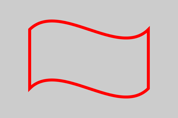
Of course, dashes don’t just apply to straight lines. We can apply a dashed lines to the outline of our Bezier shape from before:

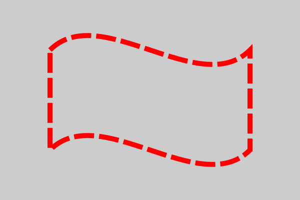
This is exactly the same code as the original Bezier example, but with a dash of [40, 10] applied. Notice that the dashes follow the curves, and even flow around the corners.