Using TensorFlow for Implementing Deep Neural Networks

There are several open source libraries and frameworks for implementing deep learning neural networks. We will look at two examples in this chapter: processing numeric cancer data to build a predictive model and for using a convolutional network for text classification. Many deep learning examples you might see on the web use image recognition as an example application but I allow myself to concentrate here on two types of problems that I use deep learning networks in my own work. In the original edition of this book both of these examples used TensorFlow; in this revised edition, I use the higher-level Keras APIs with a TensorFlow backend in the first example.

It is worth mentioning other good deep learning toolkits:

• Keras is a high level library for specifying deep networks and can use the lower level Tensorflow and Theano as back ends. Keras is especially good for rapidly prototyping different network architectures. Recommended!
• Theano is a lower level library that supports both CPU and GPU execution models.
• Caffe is a widely used C++ library for using deep neural netowkrs for image recognition.
• mxnet is another widely used deep learning library written in C++. One useful feature is language bindings for Python, R, Julia, Scala, Go, and Javascript.
• Deeplearning4j (Deep Learning for Java) is a library written for the JVM. I covered Deeplearning4j in my book Power Java with examples for deep belief networks. I especially like DeepLearning4j for deployment in production environments that use the JVM platform.

Installing TensorFlow and Keras

We will use Python 3.9 for examples in this book. Check Appendix A for detailed installation instructions. After working through the examples in this chapter, you may want to read through and experiment with Google’s TensorFlow examples as well as the examples on the Keras website.

Processing Cancer Data With a BackPropagation Network

This example is found in the subdirectory tensorflow_examples/cancer_deep_learning_model in the github repository for this book. We will use the Universary of Wisconsin Cancer Data that is in the file train.csv that has the following format:

- 0 Clump Thickness               1 - 10
- 1 Uniformity of Cell Size       1 - 10
- 2 Uniformity of Cell Shape      1 - 10
- 3 Marginal Adhesion             1 - 10
- 4 Single Epithelial Cell Size   1 - 10
- 5 Bare Nuclei                   1 - 10
- 6 Bland Chromatin               1 - 10
- 7 Normal Nucleoli               1 - 10
- 8 Mitoses                       1 - 10
- 9 Class (0 for benign, 1 for malignant)

We will use a feedforward network with two hidden layers, each hidden layer containing twelve fully connected neurons. A single output layer neuron using the sigmoid activation function will have values in the range zero to one. The network will be trained to output a small (close to zero) value for input non-cancer samples and output large values (close to one) for malignant input samples. In the following listing, lines 1-4 import the Keras (which requires and imports Tensorflow) and pandas libraires. The pandas library is using to read and write arrays as well as provide matrix operations. Pandas requires and loads the numy library that supplies data types and functionality for handling matrix operations.

We will train the network using the file train.csv and then test the trained network with different data defined in the file test.csv. We load these two datafiles using the pandas library in lines 7-12.

In lines 14-18 we define the Keras sequential model. We add two dense (i.e., fully connected) layers with shapes (9,12) and (12,12) and an output layer with a single neuron whose value is taken as the probability that an input sample is malignant. The first two hidden layers use a ReLU activation function which is now more often used than a Sigmoid activation function because of more efficient gradient propagation that helps prevent vanishing or exploding gradient problems during training. The output of a Sigmoid activation can be interpreted as a probability between zero and one and using Sigmoid function activation in the output layer is fairly much a standard procedure.

Keras allows us to register callbacks to save the model, create log data for TensorBoard visualization, early stopping of training, etc. Here we create a callback in lines 24-25 to write log data for TensorBoard.

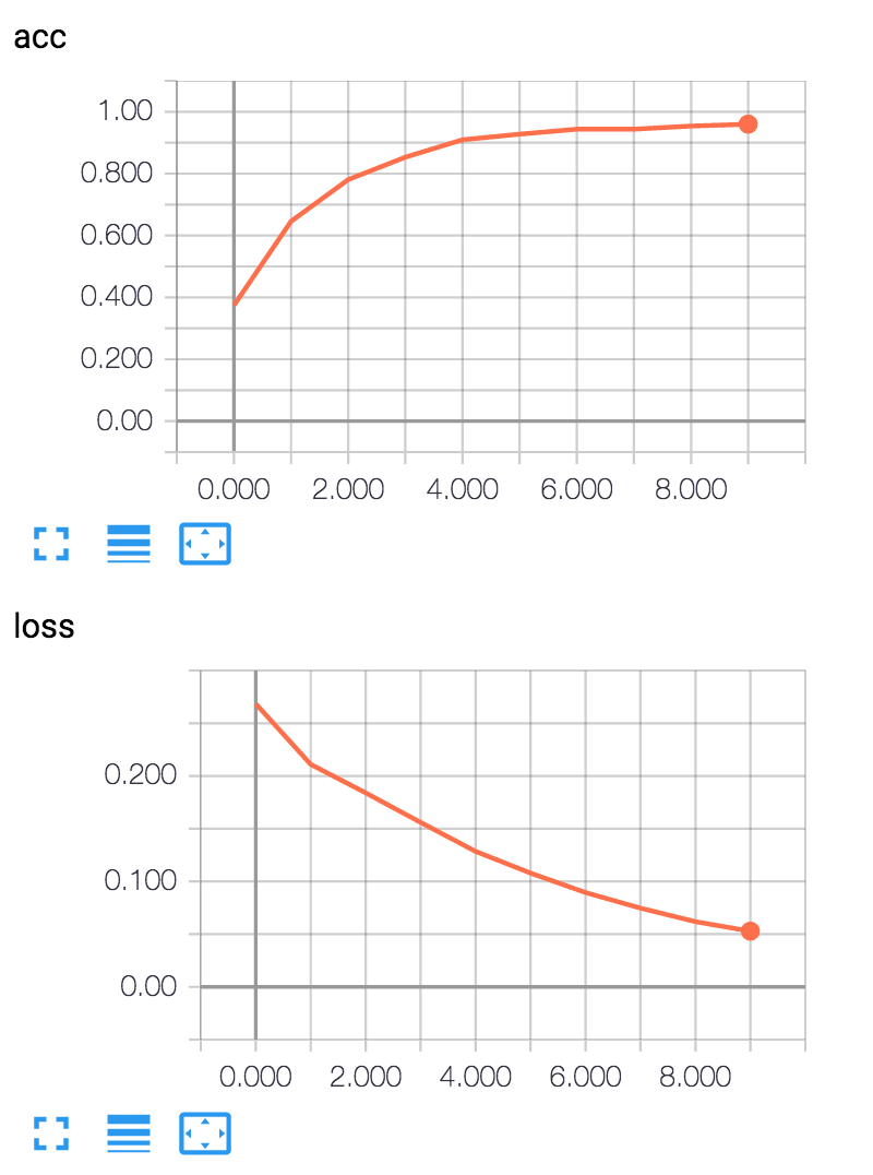
We use the trained model with the test.csv test set icalculate the accuracy over all samples in the test data (Accuracy: 0.96) and in lines 32 I show you how to use the trained model with arbitrary new test data.

TBD: update the following example

 1 from keras.models import Sequential # Keras by default imports Tensorflow
 2 from keras.layers import Dense
 3 from keras import optimizers
 4 from keras.callbacks import TensorBoard
 5 import pandas
 6 
 7 train = pandas.read_csv("train.csv", header=None).values
 8 X_train = train[:,0:9].astype(float) # 9 inputs
 9 Y_train = train[:,-1].astype(float)  # target output (0 no cancer, 1 malignant)
10 test = pandas.read_csv("test.csv", header=None).values
11 X_test = test[:,0:9].astype(float)
12 Y_test = test[:,-1].astype(float)
13 
14 model = Sequential()
15 model.add(Dense(12, input_dim=9, activation='relu'))
16 model.add(Dense(12, input_dim=12, activation='relu'))
17 model.add(Dense(1, activation='sigmoid'))
18 model.summary()
19 
20 model.compile(optimizer=optimizers.RMSprop(lr=0.002),
21               loss='mse',
22               metrics=['accuracy'])
23 
24 callbacks = [TensorBoard(log_dir='logdir', histogram_freq=0,
25                          write_graph=True, write_images=False)]
26 
27 model.fit(X_train, Y_train, batch_size=24, epochs=10, callbacks=callbacks)
28 
29 # no cancer and malignant test samples:
30 y_predict = model.predict([[4,1,1,3,2,1,3,1,1], [3,7,7,4,4,9,4,8,1]])
31 
32 print("* y_predict (should be close to [0, 1]):", y_predict)

I assume that you have TensorFlow and Keras installed. Run the example using:

 1 cancer_deep_learning_model$  export TF_CPP_MIN_LOG_LEVEL=2
 2 cancer_deep_learning_model$  source activate tensorflow27
 3 (tensorflow) cancer_deep_learning_model$ python cancer_trainer.py
 4 Using TensorFlow backend.
 5 _________________________________________________________________
 6 Layer (type)                 Output Shape              Param #   
 7 =================================================================
 8 dense_1 (Dense)              (None, 12)                120       
 9 _________________________________________________________________
10 dense_2 (Dense)              (None, 12)                156       
11 _________________________________________________________________
12 dense_3 (Dense)              (None, 1)                 13        
13 =================================================================
14 Total params: 289
15 Trainable params: 289
16 Non-trainable params: 0
17 _________________________________________________________________
18 Epoch 1/10
19 497/497 [==============================] - 0s - loss: 0.2684 - acc: 0.3742     
20 Epoch 2/10
21 497/497 [==============================] - 0s - loss: 0.2110 - acc: 0.6459     
22 Epoch 3/10
23 497/497 [==============================] - 0s - loss: 0.1840 - acc: 0.7807     
24 Epoch 4/10
25 497/497 [==============================] - 0s - loss: 0.1559 - acc: 0.8531     
26 Epoch 5/10
27 497/497 [==============================] - 0s - loss: 0.1285 - acc: 0.9095     
28 Epoch 6/10
29 497/497 [==============================] - 0s - loss: 0.1079 - acc: 0.9276     
30 Epoch 7/10
31 497/497 [==============================] - 0s - loss: 0.0894 - acc: 0.9437     
32 Epoch 8/10
33 497/497 [==============================] - 0s - loss: 0.0747 - acc: 0.9437     
34 Epoch 9/10
35 497/497 [==============================] - 0s - loss: 0.0618 - acc: 0.9537     
36 Epoch 10/10
37 497/497 [==============================] - 0s - loss: 0.0528 - acc: 0.9598     
38 * y_predict (should be close to [0, 1]): [[ 0.10986128]
39  [ 0.99367613]]

We can use the tensorbard utility (installed with Tensorflow) to look at the status of the loss function during training:

tensorboard –logdir=logdir –port=8080

If you open a web browser to http://localhost:8080 you will get the interactive TensorBoard display.

Deep Learning Wrap Up

The tutorials at tensorflow.org provide many examples of using TensorFlow. Deep learning neural networks have rapidly advanced state of the art performance in many application areas. At the natural language processing conference NAACL 2016, it seemed that about half the papers reported results using deep learning neural networks.

Regardless of your application, you are likely to find both academic papers and example systems solving similar problems using Tesnsorflow or other deep learning libraries. I recommend that you also look at Google’s Tensorflow examples.

Two other learning resources that I strongly recommend are:

• The five course Deep Learning series by Andrew Ng produced by Coursera and deeplearning.ai
• A new book by Francois Chollet who is the author of Keras: Deep Learning with Python that is a great resource for using Keras to solve practical deep learning problems.

In the next chapter we continue to look at examples of natural language processing using more conventional maximum entropy machine learning models.