8 Trees
Balancing a binary tree is the infamous interview problem that has all that folklore and debate associated with it. To tell you the truth, like the other 99% of programmers, I never had to perform this task for some work-related project. And not even due to the existence of ready-made libraries, but because self-balancing binary trees are, actually, pretty rarely used. But trees, in general, are ubiquitous even if you may not recognize their presence. The source code we operate with, at some stage of its life, is represented as a tree (a popular term here is Abstract Syntax Tree or AST, but the abstract variant is not the only one the compilers process). The directory structure of the file system is the tree. The object-oriented class hierarchy is likewise. And so on. So, returning to interview questions, trees indeed are a good area as they allow to cover a number of basic points: linked data structures, recursion, complexity. But there’s a much better task, which I have encountered a lot in practice and also used quite successfully in the interview process: breadth-first tree traversal. We’ll talk about it a bit later.
Similar to how hash-tables can be thought of as more sophisticated arrays (they are sometimes even called “associative arrays”), trees may be considered an expansion of linked lists. Although technically, a few specific trees are implemented not as a linked data structure but are based on arrays, the majority of trees are linked. Like hash-tables, some trees also allow for efficient access to the element by key, representing an alternative key-value implementation option.
Basically, a tree is a recursive data structure that consists of nodes. Each node may have zero or more children. If the node doesn’t have a parent, it is called the root of the tree. And the constraint on trees is that the root is always single. Graphs may be considered a generalization of trees that don’t impose this constraint, and we’ll discuss them in a separate chapter. In graph terms, a tree is an acyclic directed single-component graph. Directed means that there’s a one-way parent-child relation. And acyclic means that a child can’t have a connection to the parent either directly, or through some other nodes (in the opposite case, what will be the parent and what — the child?) The recursive nature of trees manifests in the fact that if we extract an arbitrary node of the tree with all of its descendants, the resulting part will remain a tree. We can call it a subtree. Besides parent-child or, more generally, ancestor-descendant “vertical” relationships that apply to all the nodes in the tree, we can also talk about horizontal siblings — the set of nodes that have the same parent/ancestor.
Another important tree concept is the distinction between terminal (leaf) and nonterminal (branch) nodes. Leaf nodes don’t have any children. In some trees, the data is stored only in the leaves with branch nodes serving to structure the tree in a certain manner. In other trees, the data is stored in all nodes without any distinction.
Implementation Variants
As we said, the default tree implementation is a linked structure. A linked list may be considered a degenerate tree with all nodes having a single child. A tree node may have more than one child, and so, in a linked representation, each tree root or subroot is the origin of a number of linked lists (sometimes, they are called “paths”).
Tree:  a
      / \
     b   c
    / \   \
   d   e   f

Lists:
a -> b -> d
a -> b -> e
a -> c -> f
b -> d
b -> e
c -> f
So, a simple linked tree implementation will look a lot like a linked list one:
(defstruct (tree-node (:conc-name nil))
  key
  children)  ; instead of linked list's next

CL-USER> (rtl:with ((f (make-tree-node :key "f"))
                    (e (make-tree-node :key "e"))
                    (d (make-tree-node :key "d"))
                    (c (make-tree-node :key "c" :children (list f)))
                    (b (make-tree-node :key "b" :children (list d e))))
            (make-tree-node :key "a"
                            :children (list b c)))
#S(TREE-NODE
   :KEY "a"
   :CHILDREN (#S(TREE-NODE
                 :KEY "b"
                 :CHILDREN (#S(TREE-NODE :KEY "d" :CHILDREN NIL)
                            #S(TREE-NODE :KEY "e" :CHILDREN NIL)))
              #S(TREE-NODE
                 :KEY "c"
                 :CHILDREN (#S(TREE-NODE :KEY "f" :CHILDREN NIL)))))
Similar to lists that had to be constructed from tail to head, we had to populate the tree in reverse order: from leaves to root. With lists, we could, as an alternative, use push and reverse the result, in the end. But, for trees, there’s no such operation as reverse.
Obviously, not only lists can be used as a data structure to hold the children. When the number of children is fixed (for example, in a binary tree), they may be defined as separate slots: e.g. left and right. Another option will be to use a key-value, which allows assigning labels to tree edges (as the keys of the kv), but the downside is that the ordering isn’t defined (unless we use an ordered kv like a linked hash-table). We may also want to assign weights or other properties to the edges, and, in this case, either an additional collection (say child-weights) or a separate edge struct should be defined to store all those properties. In the latter case, the node structure will contain edges instead of children. In fact, the tree can also be represented as a list of such edge structures, although this approach is quite inefficient, for most of the use cases.
Another tree representation utilizes the available linked list implementation directly instead of re-implementing it. Let’s consider the following simple Lisp form:
(defun foo (bar)
  "Foo function."
  (baz bar))
It is a tree with the root containing the symbol defun and 4 children:
- the terminal symbol
foo - the tree containing the function arguments (
(bar)) - the terminal sting (the docstring “Foo function.”)
- and the tree containing the form to evaluate (
(baz bar))
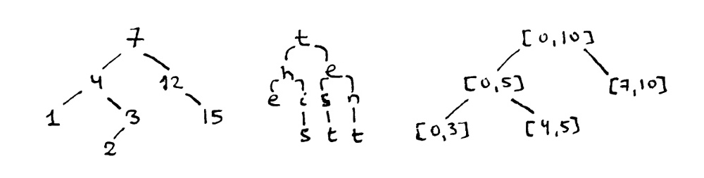
By default, in the list-based tree, the first element is the head and the rest are the leaves. This representation is very compact and convenient for humans, so it is used not only for source code. For example, you can see a similar representation for the constituency trees, in linguistics:
It is equivalent to the following parse tree:
Another, more specific, alternative is when we are interested only in the terminal nodes. In that case, there will be no explicit root and each list item will be a subtree. The following trees are equivalent:
A tree that has all terminals at the same depth and all nonterminal nodes present — a complete tree — with a specified number of children may be stored in a vector. This is a very efficient implementation that we’ll have a glance at when we talk about heaps.
Finally, a tree may be also represented, although quite inefficiently, with a matrix (only one half is necessary).
Tree Traversal
It should be noted that, unlike with other structures, basic operations, such as tree construction, modification, element search and retrieval, work differently for different tree variants. Thus we’ll discuss them further when describing those variants.
Yet, one tree-specific operation is common to all tree representations: traversal. Traversing a tree means iterating over its subtrees or nodes in a certain order. The most direct traversal is called depth-first search or DFS. It is the recursive traversal from parent to child and then to the next child after we return from the recursion. The simplest DFS for our tree-node-based tree may be coded in the following manner:
(defun dfs-node (fn root)
  (funcall fn (key root))
  (dolist (child (children root))
    (dfs-node fn child)))

;; Here, *tree* is taken from the previous example
CL-USER> (dfs-node 'print *tree*)
"a"
"b"
"d"
"e"
"c"
"f"
In the spirit of Lisp, we could also define a convenience macro:
(defmacro dotree-dfs ((value root) &body body)
  (let ((node (gensym)))  ; GENSYM is a fresh symbol
                          ; used to prevent possible symbol
                          ; collisions for NODE
    `(dfs-node (lambda (,node)
                 (let ((,value (key ,node)))
                    ,@body))
               ,root)))
And if we’d like to traverse a tree represented as a list, the changes are minor:
(defun dfs-list (fn tree)
  ;; we need to handle both subtrees (lists) and
  ;; leaves (atoms) — so, we'll just convert
  ;; everything to a list
  (let ((tree (rtl:mklist tree)))
    (funcall fn (first tree))
    (dolist (child (rest tree))
      (dfs-list fn child))))

CL-USER> (dfs-list 'print '(defun foo (bar)
                             "Foo function."
                             (baz bar)))
DEFUN
FOO
BAR
"Foo function."
BAZ
BAR
Recursion is very natural in tree traversal: we could even say that trees are recursion realized in a data structure. And the good news here is that, very rarely, there’s a chance to hit recursion limits as the majority of trees are not infinite, and also the height of the tree, which conditions the depth of recursion, grows proportionally to the logarithm of the tree size,1 and that’s pretty slow.
These simple DFS implementations apply the function before descending down the tree. This style is called preorder traversal. There are alternative styles: inorder and postorder. With postorder, the call is executed after the recursion returns, i.e. on the recursive ascent:
(defun post-dfs (fn node)
  (dolist (child (children node))
    (post-dfs fn child))
  (funcall fn (key node)))

CL-USER> (post-dfs 'print *tree*)
"d"
"e"
"b"
"f"
"c"
"a"
Inorder traversal is applicable only to binary trees: first traverse the left side, then call fn and then descend into the right side.
An alternative traversal approach is Breadth-first search (BFS). It isn’t so natural as DFS as it traverses the tree layer by layer, i.e. it has to, first, accumulate all the nodes that have the same depth and then integrate them. In the general case, it isn’t justified, but there’s a number of algorithms where exactly such ordering is required.
Here is an implementation of BFS (preorder) for our tree-nodes:
(defun bfs (fn nodes)
  (let ((next-level (list)))
    (dolist (node (rtl:mklist nodes))
      (funcall fn (key node))
      (dolist (child (children node))
        (push child next-level)))
    (when next-level
      (bfs fn (reverse next-level)))))

CL-USER> (bfs 'print *tree*)
"a"
"b"
"c"
"d"
"e"
"f"
An advantage of BFS traversal is that it can handle potentially unbounded trees, i.e. it is suitable for processing trees in a streamed manner, layer-by-layer.
In object-orientation, tree traversal is usually accomplished with by the means of the so-called Visitor pattern. Basically, it’s the same approach of passing a function to the traversal procedure but in disguise of additional (and excessive) OO-related machinery. Here is a Visitor pattern example in Java:
interface ITreeVisitor {
   List<ITreeNode> children;
   void visit(ITreeNode node);
}

interface ITreeNode {
   void accept(ITreeVisitor visitor);
}

interface IFn {
   void call(ITreeNode);
}

class TreeNode implements ITreeNode {
   public void accept(ITreeVisitor visitor) {
      visitor.visit(this);
   }
}

class PreOrderTreeVisitor implements ITreeVisitor {
   private IFn fn;

   public PreOrderTreeVisitor(IFn fn) {
        this.fn = fn;
   }

   public void visit(ITreeNode node) {
       fn.call(node);
       for (ITreeeNode child : node.children())
           child.visit(this);
   }
}
The zest of this example is the implementation of the method visit that calls the function with the current node and iterates over its children by recursively applying the same visitor. You can see that it’s exactly the same as our dfs-node.
One of the interesting tree-traversal tasks is tree printing. There are many ways in which trees can be displayed. The simplest one is directory-style (like the one used by the Unix tree utility):
$ tree /etc/acpi
/etc/acpi
├── asus-wireless.sh
├── events
│   ├── asus-keyboard-backlight-down
│   ├── asus-keyboard-backlight-up
│   ├── asus-wireless-off
│   └── asus-wireless-on
└── undock.sh
It may be implemented with DFS and only requires tracking of the current level in the tree:
(defun pprint-tree-dfs (node &optional (level 0)
                             (skip-levels (make-hash-table)))
  (when (= 0 level)
    (format t "~A~%" (key node)))
  (let ((last-index (1- (length (children node)))))
    (rtl:doindex (i child (children node))
      (let ((last-child-p (= i last-index)))
        (dotimes (j level)
          (format t "~C    "
                  (if (rtl:? skip-levels j) #\Space #\│)))
        (format t "~C── ~A~%"
                (if last-child-p #\└ #\├)
                (key child))
        (setf (rtl:? skip-levels level) last-child-p)
        (pprint-tree-dfs child
                         (1+ level)
                         skip-levels))))))

CL-USER> (pprint-tree-dfs *tree*)
a
├── b
│   ├── d
│   └── e
└── c
    └── f
1+ and 1- are standard Lisp shortucts for adding/substracting 1 from a number. The skip-levels argument is used for the last elements to not print the excess │.
A more complicated variant is top-to-bottom printing:
;; example from CL-NLP library
CL-USER> (nlp:pprint-tree
          '(TOP (S (NP (NN "This"))
                   (VP (VBZ "is")
                       (NP (DT "a")
                           (JJ "simple")
                           (NN "test")))
                   (|.| ".")))
           TOP
            :
            S
  .-----------:---------.
  :          VP         :
  :   .---------.       :
 NP   :        NP       :
  :   :   .----:-----.  :
 NN  VBZ DT   JJ    NN  .
  :   :   :    :     :  :
This  is  a simple test .
This style, most probably, will need a BFS and a careful calculation of spans of each node to properly align everything. Implementing such a function is left as an exercise to the reader, and a very enlightening one, I should say.
Binary Search Trees
Now, we can return to the topic of basic operations on tree elements. The advantage of trees is that, when built properly, they guarantee O(log n) for all the main operations: search, insertion, modification, and deletion.
This quality is achieved by keeping the leaves sorted and the trees in a balanced state. “Balanced” means that any pair of paths from the root to the leaves have lengths that may differ by at most some predefined quantity: ideally, just 1 (AVL trees), or, as in the case of Red-Black trees, the longest path can be at most twice as long as the shortest. Yet, such situations when all the elements align along a single path, effectively, turning the tree into a list, should be completely ruled out. We have already seen, with Binary search and Quicksort (remember the justification for the 3-medians rule), why this constraint guarantees logarithmic complexity.
The classic example of balanced trees are Binary Search Trees (BSTs), of which AVL and Red-Black trees are the most popular variants. All the properties of BSTs may be trivially extended to n-ary trees, so we’ll discuss the topic using the binary trees examples.
Just to reiterate the general intuition for the logarithmic complexity of tree operations, let’s examine a complete binary tree: a tree that has all levels completely filled with elements, except maybe for the last one. In it, we have n elements, and each level contains twice as many nodes as the previous. This property means that n is not greater than (+ 1 2 4 ... (/ k 2) k), where k is the capacity of the last level. This formula is nothing but the sum of a geometric progression with the number of items equal to h, which is, by the textbook:
(/ (* 1 (- 1 (expt 2 h)))
   (- 1 2))
In turn, thisexpression may be reduced to: (- (expt 2 h) 1). So (+ n 1) equals to (expt 2 h), i.e. the height of the tree (h) equals to (log (+ n 1) 2).
BSTs have the ordering property: if some element is to the right of another in the tree, it should consistently be greater (or smaller — depending on the ordering direction). This constraint means that after the tree is built, just extracting its elements by performing an inorder DFS produces a sorted sequence. The Treesort algorithm utilizes this approach directly to achieve the same O(n * log n) complexity as other efficient sorting algorithms. This n * log n is the complexity of each insertion (O(log n)) multiplied by the number of times it should be performed (n). So, Treesort operates by taking a sequence and adding its elements to the BST, then traversing the tree and putting the encountered elements into the resulting array, in a proper order.
Besides, the ordering property also means that, after adding a new element to the tree, in the general case, it should be rebalanced as the newly added element may not be placed in an arbitrary spot, but has just two admissible locations, and choosing either of those may violate the balance constraint. The specific balance invariants and approaches to tree rebalancing are the distinctive properties of each variant of BSTs that we will see below.
Splay Trees
A Splay tree represents a kind of BST that is one of the simplest to understand and to implement. It is also quite useful in practice. It has the least strict constraints and a nice property that recently accessed elements occur near the root. Thus, a Splay tree can naturally act as an LRU-cache. However, there are degraded scenarios that result in O(n) access performance, although, the average complexity of Splay tree operations is O(log n) due to amortization (we’ll talk about it in a bit).
The approach to balancing a Splay tree is to move the element we have accessed/inserted into the root position. The movement is performed by a series of operations that are called tree rotations. A certain pattern of rotations forms a step of the algorithm. For all BSTs, there are just two possible tree rotations, and they serve as the basic block, in all balancing algorithms. A rotation may be either a left or a right one. Their purpose is to put the left or the right child into the position of its parent, preserving the order of all the other child elements. The rotations can be illustrated by the following diagrams in which x is the parent node, y is the target child node that will become the new parent, and A,B,C are subtrees. It is said that the rotation is performed around the edge x -> y.
Left rotation:
Right rotation:
As you see, the left and right rotations are complementary operations, i.e. performing one after the other will return the tree to the original state. During the rotation, the inner subtree (B) has its parent changed from y to x.
Here’s an implementation of rotations:
(defstruct (bst-node (:conc-name nil)
                     (:print-object (lambda (node out)
                                      (format out "[~a-~@[~a~]-~@[~a~]]"
                                              (key node)
                                              (lt node)
                                              (rt node)))))
  key
  val  ; we won't use this slot in the examples,
       ; but without it, in real-world use cases,
       ; such a tree doesn't have any value ;)
  lt   ; left child
  rt)  ; right child

(defun tree-rotate (node parent grandparent)
  (cond
    ((eql node (lt parent)) (setf (lt parent) (rt node)
                                  (rt node) parent))
    ((eql node (rt parent)) (setf (rt parent) (lt node)
                                  (lt node) parent))
    (t (error "NODE (~A) is not the child of PARENT (~A)"
              node parent)))
  (cond
    ((null grandparent) (return-from tree-rotate node))
    ((eql parent (lt grandparent)) (setf (lt grandparent) node))
    ((eql parent (rt grandparent)) (setf (rt grandparent) node))
    (t (error "PARENT (~A) is not the child of GRANDPARENT (~A)"
              parent grandparent))))
You have probably noticed that we need to pass to this function not only the nodes on the edge around which the rotation is executed but also the grandparent node of the target to link the changes to the tree. If grandparent is not supplied, it is assumed that parent is the root and we need to separately reassign the variable holding the reference to the tree to child, after the rotation.
Splay trees combine rotations into three possible actions:
- The Zig step is used to make the node the new root when it’s already the direct child of the root. It is accomplished by a single left/right rotation(depending on whether the target is to the left or to the right of the
root) followed by an assignment. - The Zig-zig step is a combination of two zig steps that is performed when both the target node and its parent are left/right nodes. The first rotation is around the edge between the target node and its parent, and the second — around the target and its former grandparent that has become its new parent, after the first rotation.
- The Zig-zag step is performed when the target and its parent are not in the same direction: either one is left while the other is right or vise versa. In this case, correspondingly, first a left rotation around the parent is needed, and then a right one around its former grandparent (that has now become the new parent of the target). Or vice versa.
However, with our implementation of tree rotations, we don’t have to distinguish the three different steps as they are all handled at once, and so the implementation of the operation splay becomes really trivial:
(defun splay (node &rest chain)
  (loop :for (parent grandparent) :on chain :do
    (tree-rotate node parent grandparent))
  node)
The key point here and in the implementation of Splay tree operations is the use of reverse chains of nodes from the child to the root which will allow performing chains of splay operations in an end-to-end manner and also custom modifications of the tree structure.
From the code, it is clear that splaying requires at maximum the same number of steps as the height of the tree because each rotation brings the target element 1 level up. Now, let’s discuss why all Splay tree operations are O(log n). Element access requires binary search for the element in the tree, which is O(log n) provided the tree is balanced, and then splaying it to root — also O(log n). Deletion requires searching, then swapping the element either with the rightmost child of its left subtree or the leftmost child of its right subtree (direct predecessor/successor) — to make it childless, removing it, and, finally, splaying the parent of the removed node. And update is, at worst, deletion followed by insertion.
Here is the implementation of the Splay tree built of bst-nodes and restricted to only arithmetic comparison operations. All of the high-level functions, such as st-search, st-insert or st-delete return the new tree root obtained after that should substitute the previous one in the caller code.
(defun node-chain (item root &optional chain)
  "Return as the values the node equal to ITEM or the closest one to it
   and the chain of nodes leading to it, in the splay tree based in ROOT."
  (if root
      (with-slots (key lt rt) root
        (let ((chain (cons root chain)))
          (cond ((= item key) (values root
                                      chain))
                ((< item key) (st-search item lt chain))
                ((> item key) (st-search item rt chain)))))
      (values nil
              chain)))

(defun st-search (item root)
  (rtl:with ((node chain (node-chain item root)))
    (when node
      (apply 'splay chain))))

(defun st-insert (item root)
  (assert root nil "Can't insert item into a null tree")
  (rtl:with ((node chain (st-search item root)))
    (unless node
      (let ((parent (first chain)))
        ;; here, we use the property of the := expression
        ;; that it returns the item being set
        (push (setf (rtl:? parent (if (> (key parent) item)
                                      'lt
                                      'rt))
                    (make-bst-node :key item))
               chain)))
    (apply 'splay chain)))

(defun idir (dir)
  (case dir
    (rtl:lt 'rt)
    (rtl:rt 'lt)))

(defun closest-child (node)
  (dolist (dir '(lt rt))
    (let ((parent nil)
          (current nil))
      (do ((child (funcall dir node) (funcall (idir dir) child)))
          ((null child) (when current
                          (return-from closest-child
                            (values dir
                                    current
                                    parent))))
        (setf parent current
              current child)))))

(defun st-delete (item root)
  (rtl:with ((node chain (st-search item root))
             (parent (second chain)))
    (if (null node)
        root  ; ITEM was not found
        (rtl:with ((dir child child-parent (closest-child node))
                   (idir (idir dir)))
          (when parent
            (setf (rtl:? parent (if (eql (lt parent) node)
                                    'lt
                                    'rt))
                  child))
          (when child
            (setf (rtl:? child idir) (rtl:? node idir))
            (when child-parent
              (setf (rtl:? child-parent idir) (rtl:? child dir))))
          (if parent
              (apply 'splay (rest chain))
              child)))))

(defun st-update (old new root)
  (st-insert new (st-delete old root)))
The deletion is somewhat tricky due to the need to account for different cases: when removing the root, the direct child of the root, or the other node.
Let’s test the Splay tree operation in the REPL (coding pprint-bst as a slight modification of pprint-tree-dfs is left as an excercise to the reader):
CL-USER> (defparameter *st* (make-bst-node :key 5))
CL-USER> *st*
[5--]
CL-USER> (pprint-bst (setf *st* (st-insert 1 *st*)))
1
├──.
└── 5
CL-USER> (pprint-bst (setf *st* (st-insert 10 *st*)))
10
├── 1
│    ├── .
│    └── 5
└── .
CL-USER> (pprint-bst (setf *st* (st-insert 3 *st*)))
3
├── 1
└── 10
     ├── .
     └── 5
CL-USER> (pprint-bst (setf *st* (st-insert 7 *st*)))
7
├── 3
│    ├── 1
│    └── 5
└── 10
CL-USER> (pprint-bst (setf *st* (st-insert 8 *st*)))
8
├── 7
│    ├── 3
│    │    ├── 1
│    │    └── 5
│    └── .
└── 10
CL-USER> (pprint-bst (setf *st* (st-insert 2 *st*)))
2
├── 1
└── 8
     ├── 7
     │    ├── 3
     │    │    ├── .
     │    │    └── 5
     │    └── .
     └── 10
CL-USER> (pprint-bst (setf *st* (st-insert 4 *st*)))
4
├── 2
│    ├── 1
│    └── 3
└── 8
     ├── 7
     │    ├── 5
     │    └── .
     └── 10
CL-USER> *st*
[4-[2-[1--]-[3--]]-[8-[7-[5--]-]-[10--]]]
As you can see, the tree gets constantly rearranged at every insertion.
Accessing an element, when it’s found in the tree, also triggers tree restructuring:
CL-USER> (pprint-bst (st-search 5 *st*))
5
├── 4
│    ├── 2
│    │    ├── 1
│    │    └── 3
│    └── .
└── 8
     ├── 7
     └── 10
The insertion and deletion operations, for the Splay tree, also may have an alternative implementation: first, split the tree in two at the place of the element to be added/removed and then combine them. For insertion, the combination is performed by making the new element the root and linking the previously split subtrees to its left and right. As for deletion, splitting the Splay tree requires splaying the target element and then breaking the two subtrees apart (removing the target that has become the root). The combination is also O(log n) and it is performed by splaying the rightmost node of the left subtree (the largest element) so that it doesn’t have the right child. Then the right subtree can be linked to this vacant slot.
Although regular access to the Splay tree requires splaying of the element we have touched, tree traversal should be implemented without splaying. Or rather, just the normal DFS/BFS procedures should be used. First of all, this approach will keep the complexity of the operation at O(n) without the unnecessary log n multiplier added by the splaying operations. Besides, accessing all the elements inorder will trigger the edge-case scenario and turn the Splay tree into a list — exactly the situation we want to avoid.
Complexity Analysis
All of those considerations apply under the assumption that all the tree operations are O(log n). But we haven’t proven it yet. Turns out that, for Splay trees, it isn’t a trivial task and requires amortized analysis. Basically, this approach averages the cost of all operations over all tree elements. Amortized analysis allows us to confidently use many advanced data structures for which it isn’t possible to prove the required time bounds for individual operations, but the general performance over the lifetime of the data structure is in those bounds.
The principal tool of the amortized analysis is the potential method. Its idea is to combine, for each operation, not only its direct cost but also the change to the potential cost of other operations that it brings. For Splay trees, we can observe that only zig-zig and zig-zag steps are important, for the analysis, as zig step happens only once for each splay operation and changes the height of the tree by at most 1. Also, both zig-zig and zig-zag have the same potential.
Rigorously calculating the exact potential requires a number of mathematical proofs that we don’t have space to show here, so let’s just list the main results.
1. The potential of the whole Splay tree is the sum of the ranks of all nodes, where rank is the logarithm of the number of elements in the subtree rooted at node:
        (defun rank (node)
          (let ((size 0))
            (dotree-dfs (_ node)
              (incf size))
             (log size 2)))
2. The change of potential produced by a single zig-zig/zig-zag step can be calculated in the following manner:
        (+ (- (rank grandparent-new) (rank grandparent-old))
           (- (rank parent-new) (rank parent-old))
           (- (rank node-new) (rank node-old)))
(= (rank node-new) (rank grandparent-old))(- (+ (rank grandparent-new) (rank parent-new))
(+ (rank parent-old) (rank node-old)))
        (- (+ (rank grandparent-new) (rank node-new))
           (* 2 (rank node-old)))
(- (* 3 (- (rank node-new) (rank node-old))) 2)
(* 3 (- (rank node-new) (rank node-old)))
- When summed over the entire splay operation, this expression “telescopes” to
(* 3 (- (rank root) (rank node)))which isO(log n). Telescoping means that when we calculate the sum of the cost of all zig-zag/zig-zig steps, the inner terms cancel each other out and only the boundary ones remain. The difference in ranks is, in the worst case,log nas the rank of the root is(log n 2)and the rank of the arbitrary node is between that value and(log 1 2)(0). - Finally, the total cost for
msplay operations isO(m log n + n log n), wherem log nterm represents the total amortized cost of a sequence ofmoperations andn log nis the change in potential that it brings.
As mentioned, the above exposition is just a cursory look at the application of the potential method that skips some important details. If you want to learn more you can start with this discussion on CS Theory StackExchange.
To conclude, similar to hash-tables, the performance of Splay tree operations for a concrete element depends on the order of the insertion/removal of all the elements of the tree, i.e. it has an unpredictable (random) nature. This property is a disadvantage compared to some other BST variants that provide precise performance guarantees. Another disadvantage, in some situations, is that the tree is constantly restructured, which makes it mostly unfit for usage as a persistent data structure and also may not play well with many storage options. Yet, Splay trees are simple and, in many situations, due to their LRU-property, may be preferable over other BSTs.
Red-Black and AVL Trees
Another BST that also has similar complexity characteristics to Splay trees and, in general, a somewhat similar approach to rebalancing is the Scapegoat tree. Both of these BSTs don’t require storing any additional information about the current state of the tree, which results in the random aspect of their operation. And although it is smoothed over all the tree accesses, it may not be acceptable in some usage scenarios.
An alternative approach, if we want to exclude the random factor, is to track the tree state. Tracking may be achieved by adding just 1 bit to each tree node (as with Red-Black trees) or 2 bits, the so-called balance factors (AVL trees).2 However, for most of the high-level languages, including Lisp, we’ll need to go to great lengths or even perform low-level non-portable hacking to, actually, ensure that exactly 1 or 2 bits is spent for this data, as the standard structure implementation will allocate a whole word even for a bit-sized slot. Moreover, in C likewise, due to cache alignment, the structure will also have the size aligned to memory word boundaries. So, by and large, usually we don’t really care whether the data we’ll need to track is a single bit flag or a full integer counter.
The balance guarantee of an RB tree is that, for each node, the height of the left and right subtrees may differ by at most a factor of 2. Such boundary condition occurs when the longer path contains alternating red and black nodes, and the shorter — only black nodes. Balancing is ensured by the requirement to satisfy the following invariants:
- Each tree node is assigned a label: red or black (basically, a 1-bit flag: 0 or 1).
- The root should be black (0).
- All the leaves are also black (0). And the leaves don’t hold any data. A good implementation strategy to satisfy this property is to have a constant singleton terminal node that all preterminals will link to. (
(defparameter *rb-leaf* (make-rb-node))). - If a parent node is red (1) then both its children should be black (0). Due to mock leaves, each node has exactly 2 children.
- Every path from a given node to any of its descendant leaf nodes should contain the same number of black nodes.
So, to keep the tree in a balanced state, the insert/update/delete operations should perform rebalancing when the constraints are violated. Robert Sedgewick has proposed the simplest version of the red-black tree called the Left-Leaning Red-Black Tree (LLRB). The LLRB maintains an additional invariant that all red links must lean left except during inserts and deletes, which makes for the simplest implementation of the operations. Below, we can see the outline of the insert operation:
(defstruct (rb-node (:include bst-node) (:conc-name nil))
  (red nil :type boolean))

(defun rb-insert (item root &optional parent)
  (let ((node (make-rb-node :key item)))
    (when (null root)
      (return-from rb-insert node))
    (when (and (red (lt root))
               (red (rt root)))
      (setf (red root) (not (red root))
            (red (lt root)) nil
            (red (rt root)) nil))
    (cond ((< (key root) value)
           (setf (lt root) (rb-insert node (lt root) root)))
          ((> (key root) value)
           (setf (rt root) (rb-insert node (rt root) root))))
    (when (and (red (rt root))
               (not (red (lt root))))
      (setf (red (lt root)) (red root)
            root (tree-rotate (lt root) root parent)
            (red root) t))
    (when (and (red (lt root))
               (not (red (rt root))))
      (setf (red (rt root)) (red root)
            root (tree-rotate (rt root) root parent)
            (red root) t)))
  root)
This code is more of an outline. You can easily find the complete implementation of the RB-tree on the internet. The key here is to understand the principle of their operation. Also, we won’t discuss AVL trees, in detail. Suffice to say that they are based on the same principles but use a different set of balancing operations.
Both Red-Black and AVL trees may be used when worst-case performance guarantees are required, for example, in real-time systems. Besides, they serve a basis for implementing persistent data-structures that we’ll talk about later. The Java TreeMap and similar data structures from the standard libraries of many languages are implemented with one of these BSTs. And the implementations of them both are present in the Linux kernel and are used as data structures for various queues.
OK, now you know how to balance a binary tree :D
B-Trees
B-tree is a generalization of a BST that allows for more than two children. The number of children is not unbounded and should be in a predefined range. For instance, the simplest B-tree — 2-3 tree — allows for 2 or 3 children. Such trees combine the main advantage of self-balanced trees — logarithmic access time — with the benefit of arrays — locality — the property which allows for faster cache access or retrieval from the storage. That’s why B-trees are mainly used in data storage systems. Overall, B-tree implementations perform the same trick as we saw in prod-sort: switching to sequential search when the sequence becomes small enough to fit into the cache line of the CPU.
Each internal node of a B-tree contains a number of keys. For a 2-3 tree, the number is either 1 or 2. The keys act as separation values which divide the subtrees. For example, if the keys are x and y, all the values in the leftmost subtree will be less than x, all values in the middle subtree will be between x and y, and all values in the rightmost subtree will be greater than y. Here is an example:
This tree has 4 nodes. Each node has 2 key slots and may have 0 (in the case of the leaf nodes), 2 or 3 children. The node structure for it might look like this:
(defstruct 23-node
  key1
  key2
  val1
  val2
  lt
  md
  rt)
Yet, a more general B-tree node would, probably, contain arrays for keys/values and children links:
(defstruct bt-node
  (keys (make-array *max-keys*))
  (vals (make-array *max-keys*))
  (children (make-array (1+ *max-keys*)))
The element search in a B-tree is very similar to that of a BST. Just, there will be up to *max-keys* comparisons instead of 1, in each node. Insertion is more tricky as it may require rearranging the tree items to satisfy its invariants. A B-tree is kept balanced after insertion by the procedure of splitting a would-be overfilled node, of (1+ n) keys, into two (/ n 2)-key siblings and inserting the mid-value key into the parent. That’s why, usually, the range of the number of keys in the node, in the B-tree is chosen to be between k and (* 2 k). Also, in practice, k will be pretty large: an order of 10s or even 100. Depth only increases when the root is split, maintaining balance. Similarly, a B-tree is kept balanced after deletion by merging or redistributing keys among siblings to maintain the minimum number of keys for non-root nodes. A merger reduces the number of keys in the parent potentially forcing it to merge or redistribute keys with its siblings, and so on. The depth of the tree will increase slowly as elements are added to it, but an increase in the overall depth is infrequent and results in all leaf nodes being one more node farther away from the root.
A version of B-trees that is particularly developed for storage systems and is used in a number of filesystems, such as NTFS and ext4, and databases, such as Oracle and SQLite, is B+ trees. A B+ tree can be viewed as a B-tree in which each node contains only keys (not key-value pairs), and to which an additional level is added at the bottom with linked leaves. The leaves of the B+ tree are linked to one another in a linked list, making range queries or an (ordered) iteration through the blocks simpler and more efficient. Such a property could not be achieved in a B-tree, since not all keys are present in the leaves: some are stored in the root or intermediate nodes.
However, a newer Linux file-system, developed specifically for use on the SSDs and called btrfs uses plain B-trees instead of B+ trees because the former allows implementing copy-on-write, which is needed for efficient snapshots. The issue with B+ trees is that its leaf nodes are interlinked, so if a leaf were copy-on-write, its siblings and parents would have to be as well, as would their siblings and parents and so on until the entire tree was copied. We can recall the same situation pertaining to the doubly-linked list compared to singly-linked ones. So, a modified B-tree without leaf linkage is used in btrfs, with a refcount associated with each tree node but stored in an ad-hoc free map structure.
Overall, B-trees are a very natural continuation of BSTs, so we won’t spend more time with them here. I believe, it should be clear how to deal with them, overall. Surely, there are a lot of B-tree variants that have their nuances, but those should be studied in the context of a particular problem they are considered for.
Heaps
A different variant of a binary tree is a Binary Heap. Heaps are used in many different algorithms, such as path pathfinding, encoding, minimum spanning tree, etc. They even have their own O(log n) sorting algorithm — the elegant Heapsort. In a heap, each element is either the smallest (min-heap) or the largest (max-heap) element of its subtree. It is also a complete tree and the last layer should be filled left-to-right. This invariant makes the heap well suited for keeping track of element priorities. So Priority Queues are, usually, based on heaps. Thus, it’s beneficial to be aware of the existence of this peculiar data structure.
The constraints on the heap allow representing it in a compact and efficient manner — as a simple vector. Its first element is the heap root, the second and third are its left and right children (if present) and so on, by recursion. This arrangement permits access to the parent and children of any element using the simple offset-based formulas (in which the element is identified by its index):
(defun hparent (i)
  "Calculate the index of the parent of the heap element with an index I."
  (floor (- i 1) 2))

(defun hrt (i)
  "Calculate the index of the right child of the heap element with an index I."
  (* (+ i 1) 2))

(defun hlt (i)
  "Calculate the index of the left child of the heap element with an index I."
  (- (hrt i) 1))
So, to implement a heap, we don’t need to define a custom node structure, and besides, can get to any element in O(1)! Here is the utility to rearrange an arbitrary array in a min-heap formation (in other words, we can consider a binary heap to be a special arrangement of array elements). It works by iteratively placing each element in its proper place by swapping with children until it’s larger than both of the children.
(defun heapify (vec)
  (let ((mid (floor (length vec) 2)))
    (dotimes (i mid)
      (heap-down vec (- mid i 1))))
  vec)

(defun heap-down (vec beg &optional (end (length vec)))
  (let ((l (hlt beg))
        (r (hrt beg)))
    (when (< l end)
      (let ((child (if (or (>= r end)
                           (> (aref vec l)
                              (aref vec r)))
                       l r)))
        (when (> (aref vec child)
                 (aref vec beg))
          (rotatef (aref vec beg)
                   (aref vec child))
          (heap-down vec child end)))))
  vec)
And here is the reverse operation to pop the item up the heap:
(defun heap-up (vec i)
  (when (> (aref vec i)
           (aref vec (hparent i)))
    (rotatef (aref vec i)
             (aref vec (hparent i)))
    (heap-up vec (hparent i)))
  vec)
Also, as with other data structures, it’s essential to be able to visualize the content of the heap in a convenient form, as well as to check the invariants. These tasks may be accomplished with the help of the following functions:
(defun draw-heap (vec)
  (format t "~%")
  (rtl:with ((size (length vec))
             (h (+ 1 (floor (log size 2)))))
    (dotimes (i h)
      (let ((spaces (make-list (- (expt 2 (- h i)) 1)
                          :initial-element #\Space)))
        (dotimes (j (expt 2 i))
          (let ((k (+ (expt 2 i) j -1)))
            (when (= k size) (return))
            (format t "~{~C~}~2D~{~C~}"
                    spaces (aref vec k) spaces)))
        (format t "~%"))))
  (format t "~%")
  vec)

(defun check-heap (vec)
  (dotimes (i (floor (length vec) 2))
    (when (= (hlt i) (length vec)) (return))
    (assert (not (> (aref vec (hlt i)) (aref vec i)))
            () "Left child (~A) is > parent at position ~A (~A)."
            (aref vec (hlt i)) i (aref vec i))
    (when (= (hrt i) (length vec)) (return))
    (assert (not (> (aref vec (hrt i)) (aref vec i)))
            () "Right child (~A) is > than parent at position ~A (~A)."
            (aref vec (hrt i)) i (aref vec i)))
  vec)

CL-USER> (check-heap #(10 5 8 2 3 7 1 9))
Left child (9) is > parent at position 3 (2).
   [Condition of type SIMPLE-ERROR]

CL-USER> (check-heap (draw-heap (heapify #(1 22 10 5 3 7 8 9 7 13))))

               22
       13              10
    9       3       7       8
  5   7   1

#(22 13 10 9 3 7 8 5 7 1)
Due to the regular nature of the heap, drawing it with BFS is much simpler than for most other trees.
As with ordered trees, heap element insertion and deletion require repositioning of some of the elements.
(defun heap-push (node vec)
  (vector-push-extend node vec)
  (heap-up vec (1- (length vec))))

(defun heap-pop (vec)
  (rotatef (aref vec 0) (aref vec (- (length vec) 1)))
  ;; PROG1 is used to return the result of the first form
  ;; instead of the last, like it happens with PROGN
  (prog1 (vector-pop vec)
    (heap-down vec 0)))
Now, we can implement Heapsort. The idea is to iteratively arrange the array in heap order element by element. Each arrangement will take log n time as we’re pushing the item down a complete binary tree the height of which is log n. And we’ll need to perform n such iterations.
(defun heapsort (vec)
  (heapify vec)
  (dotimes (i (length vec))
    (let ((last (- (length vec) i 1)))
      (rotatef (aref vec 0)
               (aref vec last))
      (heap-down vec 0 last)))
  vec)

CL-USER> (heapsort #(1 22 10 5 3 7 8 9 7 13))
#(1 3 5 7 7 8 9 10 13 22)
There are so many sorting algorithms, so why invent yet another one? That’s a totally valid point, but the advantage of heaps is that they keep the maximum/minimum element constantly at the top so you don’t have to perform a full sort or even descend into the tree if you need just the top element. This simplification is especially relevant if we constantly need to access such elements as with priority queues.
Actually, a heap should not necessarily be a tree. Besides the Binary Heap, there are also Binomial, Fibonacci and other kinds of heaps that may even not necessary be trees, but even collections of trees (forests). We’ll discuss some of them in more detail in the next chapters, in the context of the algorithms for which their use makes a notable difference in performance.
Tries
If I were to answer the question, what’s the most underappreciated data structure, I’d probably say, a trie. For me, tries are a gift that keeps on giving, and they have already saved me program performance in a couple of situations that seemed hopeless. Besides, they are very simple to understand and implement.
A trie is also called a prefix tree. It is, usually, used to optimize dictionary storage and lookup when the dictionary has a lot of entries and there is some overlap between them. The most obvious example is a normal English language dictionary. A lot of words have common stems (“work”, “word”, “worry” all share the same beginning “wor”), there are many wordforms of the same word (“word”, “words”, “wording”, “worded”).
Thre are many approaches to trie implementation. Let’s discuss with the most straightforward and, to so to say, primitive one. Here is a trie for representing a string dictionary that is character-based and uses an alist to store children pointers:
(defstruct (tr-node (:conc-name nil))
  val
  (children (list)))

(defun tr-lookup (key root)
  (rtl:dovec (ch key
              ;; when iteration terminates normally
              ;; we have found the node we were looking for
              (val root))
    (rtl:if-it (rtl:assoc1 ch (children root))
               (setf root rtl:it)
               (return))))

(defun tr-add (key val root)
  (let ((i 0))
    (rtl:dovec (ch key)
      (rtl:if-it (rtl:assoc1 ch (children root))
                 (setf root rtl:it
                       i (1+ i))
                 (return)))
    (if (= i (length key))
        ;; something has already being stored at key -
        ;; so we signal a continuable error that
        ;; gives the user two options: overwrite or abort
        (cerror "Assign a new value"
                "There was already a value at key: ~A" (val root))
        (rtl:dovec (ch (rtl:slice key i))
          (let ((child (make-tr-node)))
            (push (cons ch child) (children root))
            (setf root child))))
    (setf (val root) val)))

CL-USER> (defparameter *trie* (make-tr-node))
*TRIE*
CL-USER> *trie*
#S(TR-NODE :VAL NIL :CHILDREN NIL)
For the sake of brevity, we won’t define a special print-function for our trie and will use a default one. In a real setting, though, it is highly advisable.
CL-USER> (tr-lookup "word" *trie*)
NIL
CL-USER> (tr-add "word" 42 *trie*)
42
CL-USER> *trie*
#S(TR-NODE
   :VAL NIL
   :CHILDREN
   ((#\w
     . #S(TR-NODE
          :VAL NIL
          :CHILDREN
          ((#\o
            . #S(TR-NODE
                 :VAL NIL
                 :CHILDREN
                 ((#\r
                   . #S(TR-NODE
                        :VAL NIL
                        :CHILDREN
                        ((#\d
                          . #S(TR-NODE
                               :VAL 42
                               :CHILDREN NIL)))))))))))))
CL-USER> (tr-lookup "word" *trie*)
42
CL-USER> (tr-add "word" :foo *trie*)

There was already a value at key: 42
   [Condition of type SIMPLE-ERROR]

Restarts:
 0: [CONTINUE] Assign a new value
 1: [RETRY] Retry SLIME REPL evaluation request.
 2: [*ABORT] Return to SLIME's top level.
 3: [ABORT] abort thread (#<THREAD "repl-thread" RUNNING>)

Backtrace:
  0: (TR-ADD "word" :FOO #S(TR-NODE :VAL 42 :CHILDREN NIL))
  1: (SB-INT:SIMPLE-EVAL-IN-LEXENV (TR-ADD "word" :FOO *TRIE*) #<NULL-LEXENV>)
  2: (EVAL (TR-ADD "word" :FOO *TRIE*))
 --more--

;;; Take the restart 0

:FOO
CL-USER> (tr-add "we" :baz *trie*)
:BAZ
CL-USER> *trie*
#S(TR-NODE
   :VAL NIL
   :CHILDREN
   ((#\w
     . #S(TR-NODE
          :VAL NIL
          :CHILDREN
          ((#\e . #S(TR-NODE
                     :VAL :BAZ
                     :CHILDREN NIL))
           (#\o . #S(TR-NODE
                     :VAL NIL
                     :CHILDREN
                     ((#\r
                       . #S(TR-NODE
                            :VAL NIL
                            :CHILDREN
                            ((#\k
                              . #S(TR-NODE
                                   :VAL :BAR
                                   :CHILDREN NIL))
                             (#\d
                              . #S(TR-NODE
                                   :VAL :FOO
                                   :CHILDREN NIL)))))))))))))
There are many ways to optimize this trie implementation. First of all, you can see that some space is wasted on intermediate nodes with no values. This is mended by Radix Trees (also known as Patricia Trees) that merge all intermediate nodes. I.e., our trie would change into the following more compact structure:
#S(TR-NODE
   :VAL NIL
   :CHILDREN
   ((#\w
     . #S(TR-NODE
          :VAL NIL
          :CHILDREN
          ((#\e . #S(TR-NODE
                     :VAL :BAZ
                     :CHILDREN NIL))
           ("or" . #S(TR-NODE
                      :VAL NIL
                      :CHILDREN ((#\k . #S(TR-NODE
                                           :VAL :BAR
                                           :CHILDREN NIL))
                                 (#\d . #S(TR-NODE
                                           :VAL :FOO
                                           :CHILDREN NIL))))))))))
Besides, there are ways to utilize the array to store trie offsets (similar to heaps), instead of using a linked backbone for it. Such variant is called a succinct trie. Also, there are compressed (C-tries), hash-array mapped (HAMTs), and other kinds of tries.
The main advantage of tries is efficient space usage thanks to the elimination of repetition in keys storage. In many scenarios, usage of tries also improves the speed of access. Consider the task of matching against a dictionary of phrases, for example, biological or medical terms, names of companies or works of art, etc. These are usually 2-3 words long phrases, but, occasionally, there may be an outlier of 10 or more words. The straightforward approach would be to put the dictionary into a hash-table, then iterate over the input string trying to find the phrases in the table, starting from each word. The only question is: where do we put an end of the phrase? As we said, the phrase may be from 1 to, say, 10 words in length. With a hash-table, we have to check every variant: a single-word phrase, a two-word one, and so on up to the maximum length. Moreover, if there are phrases with the same beginning, which is often the case, we’d do duplicate work of hashing that beginning, for each variant (unless we use an additive hash, but this isn’t adviced for hash-tables). With a trie, all the duplication is not necessary: we can iteratively match each word until we either find the match in the tree or discover that there is no continuation of the current subphrase.
Trees in Action: Efficient Mapping
Finally, the last family of tree data structures I had to mention is trees for representing spatial relations. Overall, mapping and pathfinding is an area that prompted the creation of a wide range of useful algorithms and data structures. There are two fundamental operations for processing spatial data: nearest neighbor search and range queries. Given the points on the plane, how do we determine the closest points to a particular one? How do we retrieve all points inside a rectangle or a circle? A primitive approach is to loop through all the points and collect the relevant information, which results in at least O(n) complexity — prohibitively expensive if the number of points is beyond several tens or hundreds. And such problems, by the way, arise not only in the field of processing geospatial data (they are at the core of such systems as PostGIS, mapping libraries, etc.) but also in Machine Learning (for instance, the k-NN algorithm directly requires such calculations) and other areas.
A more efficient solution has an O(log n) complexity and is, as you might expect, based on indexing the data in a special-purpose tree. The changes to the tree will also have O(log n) complexity, while the initial indexing is O(n log n). However, in most of the applications that use this technique, changes are much less frequent than read operations, so the upfront cost pays off.
There is a number of trees that allow efficient storage of spatial data: segment trees, interval trees, k-d trees, R-trees, etc. The most common spatial data structure is an R-tree (rectangle-tree). It distributes all the points in an n-dimensional space (usually, n will be 2 or 3) among the leaves of the tree by recursively dividing the space into k rectangles holding roughly the same number of points until each tree node has at most k points.
Let’s say we have started from 1000 points on the plane and chosen k to be 10. In this case, the first level of the tree (i.e. children of the root) will contain 10 nodes, each one having as the value the dimensions of the rectangle that bounds approximately 100 points. Every node like that will have 10 more children, each one having around 10 points. Maybe, some will have more, and, in this case, we’ll give those nodes 10 children each with, probably, 1 or 2 points in the rectangles they will command. Now, we can perform a range search with the obtained tree by selecting only the nodes that intersect the query rectangle. For a small query box, this approach will result in the discarding of the majority of the nodes at each level of the tree. So, a range search over an R-tree has O(k log n) where k is the number of intersecting rectangles.
Now, let’s consider neighbor search. Obviously, the closest points to a particular one we are examining lie either in the same rectangle as the point or in the closest ones to it. So, we need to, first, find the smallest bounding rectangle, which contains our point, perform the search in it, then, if we haven’t got enough points yet, process the siblings of the current tree node in the order of their proximity to it.
There are many other spatial problems that may be efficiently solved with this approach. One thing to note is that the described procedures require the tree to store, in the leaf nodes, references to every point contained in their rectangles.
Take-Aways
So, balancing a tree isn’t such a unique and interesting task. On the contrary, it’s quite simple yet boring due to the number of edge cases you have to account for. Yet, we have just scratched the surface of the general topic of trees. It is vast: the Wikipedia section for tree data structures contains almost 100 of them and it’s, definitely, not complete. Moreover, new tree variants will surely be invented in the future. But you will hardly deal with more than just a few variants during the course of your career, spending the majority of time with the simple “unconstrained” trees. And we have seen, in action, the basic principles of tree operation that will be helpful, in the process.
There’s a couple of other general observations about programming algorithms we can draw from this chapter:
- Trees are very versatile data structures that are a default choice when you need to represent some hierarchy. They are also one of a few data structures for which recursive processing is not only admissible but also natural and efficient.
- Visualization is key to efficient debugging of complex data-structures. Unfortunately, it’s hard to show that in the book how I have spent several hours on the code for the splay tree, but without an efficient way to display the trees coupled with dynamic tracing, I would probably have spent twice as much. And, both the
print-functionfor individual node andpprint-bstwere helpful here.