9 Graphs
Graphs have already been mentioned several times in the book, in quite diverse contexts. Actually, if you are familiar with graphs you can spot opportunities to use them in quite different areas for problems that aren’t explicitly formulated with graphs in mind. So, in this chapter, we’ll discuss how to handle graphs to develop such intuition to some degree.
But first, let’s list the most prominent examples of the direct graph applications, some of which we’ll see here in action:
- pathfinding
- network analysis
- dependency analysis in planning, compilers, etc.
- various optimization problems
- distributing and optimizing computations
- knowledge representation and reasoning with it
- meaning representation in natural language processing
Graphs may be thought of as a generalization of trees: indeed, trees are, as we said earlier, connected directed acyclic graphs. But there’s an important distinction in the patterns of the usage of graphs and trees. Graphs, much more frequently than trees, have weights associated with the edges, which adds a whole new dimension both to algorithms for processing them and to possible data that can be represented in the graph form. So, while the main application of trees is reflecting some hierarchy, for graphs, it is often more about determining connectedness and its magnitude, based on the weights.
Graph Representations
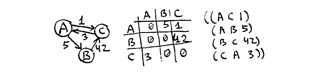
A graph is, basically, a set of nodes (called “vertices”, V) and an enumeration of connections between two nodes (“edges”, E). The edges may be directed or undirected (i.e. bidirectional), and also weighted or unweighted. There are many ways that may be used to represent these sets, which have varied utility for different situations. Here are the most common ones:
- as a linked structure:
(defstruct node data links)wherelinksmay be either a list of othernodes, possibly, paired with weights, or a list ofedgestructures represented as(defsturct edge source destination weight). For directed graphs, this representation will be similar to a singly-linked list but for undirected — to a heavier doubly-linked one - as an adjacency matrix (
V x V). This matrix is indexed by vertices and has zeroes when there’s no connection between them and some nonzero number for the weight (1 — in case of unweighted graphs) when there is a connection. Undirected graphs have a symmetric adjacency matrix and so need to store only the abovediagonal half of it - as an adjacency list that enumerates for each vertex the other vertices it’s connected to and the weights of connections
- as an incidence matrix (
V x E). This matrix is similar to the adjacency list representation but with much more wasted space. The adjacency list may be thought of as a sparse representation of the incidence matrix. The matrix representation may be more useful for hypergraphs (that have more than 2 vertices for each edge), though - just as a list of edges
Topological Sort
Graphs may be divided into several kinds according to the different properties they have and specific algorithms which work on them:
- disjoint (with several unconnected subgraphs), connected, and fully-connected (every vertex is linked to all the others)
- cyclic and acyclic, including directed acyclic (DAG)
- bipartite: when there are 2 groups of vertices and each vertex from one group is connected only to the vertices from the other
In practice, Directed Acyclic Graphs are quite important. These are directed graphs, in which there’s no vertex that you can start a path from and return back to it. They find applications in optimizing scheduling and computation, determining historical and other types of dependencies (for example, in dataflow programming and even spreadsheets), etc. In particular, every compiler would use one and even make will when building the operational plan. The basic algorithm on DAGs is Topological sort. It creates a partial ordering of the vertices of the graph which ensures that every child vertex is always preceding all of its ancestors.
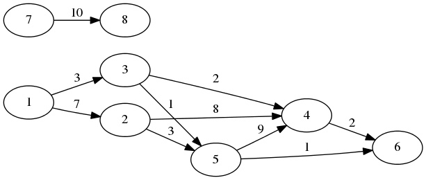
Here is an example. This is a DAG:
And these are the variants of its topological ordering:
There are several variants as the graph is disjoint, and also the order in which the vertices are traversed is not fully deterministic.
There are two common approaches to topological sort: the Kahn’s algorithm and the DFS-based one. Here is the DFS version:
- Choose an arbitrary vertex and perform the DFS from it until a vertex is found without children that weren’t visited during the DFS.
- While performing the DFS, add each vertex to the set of visited ones. Also check that the vertex hasn’t been visited already, or else the graph is not acyclic.
- Then, add the vertex we have found to the resulting sorted array.
- Return to the previous vertex and repeat searching for the next descendant that doesn’t have children and add it.
- Finally, when all of the current vertex’s children are visited add it to the result array.
- Repeat this for the next unvisited vertex until no unvisited ones remain.
Why does the algorithm satisfy the desired constraints? First of all, it is obvious that it will visit all the vertices. Next, when we add the vertex, we have already added all of its descendants — satisfying the main requirement. Finally, there’s a consistency check during the execution of the algorithm that ensures there are no cycles.
Before proceeding to the implementation, as with other graph algorithms, it makes sense to ponder what representation will work the best for this problem. The default one — a linked structure — suits it quite well as we’ll have to iterate all the outgoing edges of each node. If we had to traverse by incoming edges then it wouldn’t have worked, but a matrix one would have.
(defstruct node
  id edges)

(defstruct edge
  src dst label)

(defstruct (graph (:conc-name nil) (:print-object pprint-graph))
  (nodes (make-hash-table)))  ; mapping of node ids to nodes
As usual, we’ll need a more visual way to display the graph than the default print-function. But that is pretty tricky considering that graphs may have an arbitrary structure with possibly intersecting edges. The simplest approach for small graphs would be to just draw the adjacency matrix. We’ll utilize it for our examples (relying on the fact that we have control over the set of node ids):
(defun pprint-graph (graph stream)
  (let ((ids (sort (rtl:keys (nodes graph)) '<)))
    (format stream "~{    ~A~}~%" ids)  ; here, Tab is used for space
    (dolist (id1 ids)
      (let ((node (rtl:? graph 'nodes id1)))
        (format stream "~A" id1)
        (dolist (id2 ids)
          (format stream "    ~:[~;x~]"   ; here, Tab as well
                  (find id2 (rtl:? node 'edges) :key 'edge-dst)))
        (terpri stream)))))
Also, let’s create a function to simplify graph initialization:
(defun init-graph (edges)
  (rtl:with ((rez (make-graph))
             (nodes (nodes rez)))
    (loop :for (src dst) :in edges :do
      (let ((src-node (rtl:getsethash src nodes (make-node :id src))))
        (rtl:getset# dst nodes (make-node :id dst))
        (push (make-edge :src src :dst dst)
              (rtl:? src-node 'edges))))
    rez))

CL-USER> (init-graph '((7 8)
                       (1 3)
                       (1 2)
                       (3 4)
                       (3 5)
                       (2 4)
                       (2 5)
                       (5 4)
                       (5 6)
                       (4 6)))
So, we already see in action 3 different ways of graphs representation: linked, matrix, and edges lists.
Now, we can implement and test topological sort:
(defun topo-sort (graph)
  (let ((nodes (nodes graph))
        (visited (make-hash-table))
        (rez (rtl:vec)))
    (rtl:dokv (id node nodes)
      (unless (gethash id visited)
        (visit node nodes visited rez)))
    rez))

(defun visit (node nodes visited rez)
  (dolist (edge (node-edges node))
    (rtl:with ((id (edge-dst edge))
               (child (elt nodes id)))
      (unless (find id rez)
        (assert (not (gethash id visited)) nil
                "The graph isn't acyclic for vertex: ~A" id)
        (setf (gethash id visited) t)
        (visit child nodes visited rez))))
  (vector-push-extend (node-id node) rez)
  rez)

CL-USER> (topo-sort (init-graph '((7 8)
                                  (1 3)
                                  (1 2)
                                  (3 4)
                                  (3 5)
                                  (2 4)
                                  (2 5)
                                  (5 4)
                                  (5 6)
                                  (4 6))))
#(8 7 6 4 5 2 3 1)
This technique of tracking the visited nodes is used in almost every graph algorithm. As noted previously, it can either be implemented using an additional hash-table (like in the example) or by adding a Boolean flag to the vertex/edge structure itself.
MST
Now, we can move to algorithms that work with weighted graphs. They represent the majority of the interesting graph-based solutions. One of the most basic of them is determining the Minimum Spanning Tree. Its purpose is to select only those graph edges that form a tree with the lowest total sum of weights. Spanning trees play an important role in network routing where there is a number of protocols that directly use them: STP (Spanning Tree Protocol), RSTP (Rapid STP), MSTP (Multiple STP), etc.
If we consider the graph from the previous picture, its MST will include the edges 1-2, 1-3, 3-4, 3-5, 5-6, and 7-8. Its total weight will be 24.
Although there are quite a few MST algorithms, the most well-known are Prim’s and Kruskal’s. Both of them rely on some interesting solutions and are worth studying.
Prim’s Algorithm
Prim’s algorithm grows the tree one edge at a time, starting from an arbitrary vertex. At each step, the least-weight edge that has one of the vertices already in the MST and the other one outside is added to the tree. This algorithm always has an MST of the already processed subgraph, and when all the vertices are visited, the MST of the whole graph is completed. The most interesting property of Prim’s algorithm is that its time complexity depends on the choice of the data structure for ordering the edges by weight. The straightforward approach that searches for the shortest edge will have O(V^2) complexity, but if we use a priority queue it can be reduced to O(E logV) with a binary heap or even O(E + V logV) with a Fibonacci heap. Obviously, V logV is significantly smaller than E logV for the majority of graphs: up to E = V^2 for fully-connected graphs.
Here’s the implementation of the Prim’s algorithm with an abstract heap:
(defvar *heap-indices*)

(defun prim-mst (graph)
  (let ((initial-weights (list))
        (mst (list))
        (total 0)
        (*heap-indices* (make-hash-table))
        weights
        edges
        cur)
    (rtl:dokv (id node (nodes graph))
      (if cur
          (push (rtl:pair id (or (elt edges id)
                                 ;; a standard constant that is
                                 ;; a good enough substitute for infinity
                                 most-positive-fixnum))
                initial-weights)
          (setf cur id
                edges (node-edges node))))
    (setf weights (heapify initial-weights))
    (loop
      (rtl:with (((id weight) (heap-pop weights)))
        (unless id (return))
        (when (elt edges id)
          ;; if not, we have moved to the new connected component
          ;; so there's no edge connecting it to the previous one
          (push (rtl:pair cur id) mst)
          (incf total weight))
        (rtl:dokv (id w edges)
          (when (< w weight)
            (heap-decrease-key weights id w)))
        (setf cur id
              edges (rtl:? graph 'nodes id 'edges))))
    (values mst
            total)))
To make it work, we need to perform several modifications.
- First of all, the list of all node edges should be changed to a hash-table to ensure
O(1)access by child id. - We need to implement another fundamental heap operation
heap-decrease-key, which we haven’t mentioned in the previous chapter. For the binary heap, it’s actually just a matter of executingheap-upafter the value of a particular key is decremented. The tricky part is that it requires an initial search for the key in the heap. To ensure constant-time search and subsequentlyO(log n)total complexity, we need to store the pointers to heap elements in a separate hash-table. This is where a special variable heap-indices comes into play. All the heap operations will need to update the key positions tracked in it. Using a special vaiable may be very handy in such situations when we need to extend an existing API without breaking all the code that is already using it. Surely, we could also define a new set of heap operations (let’s call themheapify-with-tracking,heap-pop-with-tracking, etc) with an updated argument list, and we’ll have to pass the tracking hash-table around with each call. That is a more standard and “proper” solution. Yet, sometimes it is not possible to do that, and in such situations special variables provide a viable solution for retrofitting your code with new features. I won’t list here the updated code for all the heap operations that uses the new variable (you can develop it on your own as an excercise), instead we’ll just take a look at the new version of the essentialheap-downandheap-up, as well as the newly defined decrease-key operation:
    (defun heap-down (vec beg &optional (end (length vec)))
      (let ((l (hlt beg))
            (r (hrt beg)))
        (when (< l end)
          (let ((child (if (or (>= r end)
                               (> (aref vec l)
                                  (aref vec r)))
                           l r)))
            (when (> (aref vec child)
                     (aref vec beg))
              (rotatef (gethash (aref vec beg) *heap-indices*)
                       (gethash (aref vec child) *heap-indices*))
              (rotatef (aref vec beg)
                       (aref vec child))
              (heap-down vec child end)))))
      vec)

    (defun heap-up (vec i)
      (let ((parent (hparent i)))
        (when (> (aref vec i)
                 (aref vec parent))
          (rotatef (gethash (aref vec i) *heap-indices*)
                   (gethash (aref vec parent) *heap-indices*)))
          (rotatef (aref vec i)
                   (aref vec parent))
        (heap-up vec parent))
      vec)

    (defun heap-decrease-key (vec key decrement)
      (let ((i (gethash key *heap-indices*)))
        (unless i (error "No key ~A found in the heap: ~A" key vec))
        (remhash key *heap-indices*)
        (setf (gethash (- key decrement) *heap-indices*) i)
        (decf (aref vec i) decrement)
        (heap-up vec i)))
    (defun heap-decrease-key (vec key decrement)
      (let ((i (pop (gethash key *heap-indices*))))
        (unless i (error "No key ~A found in the heap: ~A" key vec))
        (when (null (gethash key *heap-indices*))
          (remhash key *heap-indices*))
        (push i (gethash (- key decrement) *heap-indices*))
        (decf (aref vec i) decrement)
        (heap-up vec i)))

    (defun heap-up (vec i)
      (rtl:with ((i-key (aref vec i))
                 (parent (hparent i))
                 (parent-key (aref vec parent)))
        (when (> i-key parent-key)
          (rtl:removef i (gethash i-key *heap-indices*))
          (rtl:removef parent (gethash parent-key *heap-indices*))
          (push i (gethash parent-key *heap-indices*))
          (push parent (gethash i-key *heap-indices*))
          (rotatef (aref vec i)
                   (aref vec parent))
        (heap-up vec parent))
      vec)

    ;; and so on and so forth
- The heap should store not only the keys but also values: another trivial but rather tedious change that will further complicate the code as, this time, we’ll have to pass around a pair or a struct instead of an index and remember to always access the key of an item instead of the item itself. Something along these lines:
(defstructheap-itemkeyval)(defunheap-up(veci)(rtl:with((i-key(heap-item-key(arefveci)))(parent(hparenti))(parent-key(heap-item-key(arefvecparent))))(when(>i-keyparent-key)(rtl:removefi(gethashi-key*heap-indices*))(rtl:removefparent(gethashparent-key*heap-indices*))(pushi(gethashparent-key*heap-indices*))(pushparent(gethashi-key*heap-indices*))(rotatef(arefveci)(arefvecparent))(heap-upvecparent))vec)
Let’s confirm the stated complexity of this implementation. First, the outer loop operates for each vertex so it has V iterations. Each iteration has an inner loop that involves a heap-pop (O(log V)) and a heap-update (also O(log V)) for a number of vertices, plus a small number of constant-time operations. heap-pop will be invoked exactly once per vertex, so it will need O(V logV) total operations, and heap-update will be called at most once for each edge (O(E logV)). Considering that E is usually greater than V, this is how we can arrive at the final complexity estimate.
Also, it’s worth noting that adding the index-bookkeeping operations to each fundamental heap reordering doesn’t change its basic logarithmic execution complexity, although it increases the hidden constant factor. Hash-table accesses are O(1) and, although rtl:removef performs a linear scan we can be sure that the number of duplicate keys over the whole execution of the algorithm will not be comparable to the number of all keys as we’re constantly perfroming the decrease key operation, so even when a batch of duplicates stochastically accumulate, such state will not persist for a long time.
The Fibonacci heap may be used to further improve the complexity characteristics of this algorithms. Its decrease-key operation is O(1) instead of O(log V), so we are left with just O(V logV) for heap-pops and E heap-decrease-keys. Unlike the binary heap, the Fibonacci one is not just a single tree but a set of trees. And this property is used in decrease-key: instead of popping an item up the heap and rearranging the vector in the process, a new tree rooted at this element is cut from the current one. This is not always possible in constant time as there are some invariants that might be violated, which will in turn trigger some updates to the newly created two trees. Yet, using amortized cost analysis, it is possible to prove that the average operation complexity is still O(1).
Here’s a brief description of the principle behind the Fibonacci heap adapted from Wikipedia:
A Fibonacci heap is a collection of heaps. The trees do not have a prescribed shape and, in the extreme case, every element may be its own separate tree. This flexibility allows some operations to be executed in a lazy manner, postponing the work for later operations. For example, merging heaps is done simply by concatenating the two lists of trees, and operation decrease key sometimes cuts a node from its parent and forms a new tree. However, at some point order needs to be introduced to the heap to achieve the desired running time. In particular, every node can have at most O(log n) children and the size of a subtree rooted in a node with k children is at least F(k+2), where F(k) is the k-th Fibonacci number. This is achieved by the rule that we can cut at most one child of each non-root node. When a second child is cut, the node itself needs to be cut from its parent and becomes the root of a new tree. The number of trees is decreased in the operation delete minimum, where trees are linked together. Here’s an example Fibonacci heap that consists of 3 trees:
6  2      1 <- minimum
   |    / | \
   5   3  4  7
             |
             8
             |
             9
Kruskal’s Algorithm
Kruskal’s algorithm operates not from the point of view of vertices but of edges. At each step, it adds to the tree the current smallest edge unless it will produce a cycle. Obviously, the biggest challenge here is to efficiently find the cycle. Yet, the good news is that, like with the Prim’s algorithm, we also have already access to an efficient solution for this problem — Union-Find. Isn’t it great that we have already built a library of techniques that may be reused in creating more advanced algorithms? Actually, this is the goal of developing as an algorithms programmer — to be able to see a way to reduce the problem, at least partially, to some already known and proven solution.
Like Prim’s algorithm, Kruskal’s approach also has O(E logV) complexity: for each vertex, it needs to find the minimum edge not forming a cycle with the already built partial MST. With Union-Find, this search requires O(logE), but, as E is at most V^2, logE is at most logV^2 that is equal to 2 logV. Unlike Prim’s algorithm, the partial MST built by the Kruskal’s algorithm isn’t necessary a tree for the already processed part of the graph.
The implementation of the algorithm, using the existing code for Union-Find is trivial and left as an exercise to the reader.
Pathfinding
So far, we have only looked at problems with unweighted graphs. Now, we can move to weighted ones. Pathfinding in graphs is a huge topic that is crucial in many domains: maps, games, networks, etc. Usually, the goal is to find the shortest path between two nodes in a directed weighted graph. Yet, there may be variations like finding shortest paths from a selected node to all other nodes, finding the shortest path in a maze (that may be represented as a grid graph with all edges of weight 1), etc.
Once again, there are two classic pathfinding algorithms, each one with a certain feature that makes it interesting and notable. Dijkstra’s algorithm is a classic example of greedy algorithms as its alternative name suggests — shortest path first (SPF). The A* builds upon it by adding the notion of an heuristic. Dijkstra’s approach is the basis of many computer network routing algorithms, such as IS-IS and OSPF, while A* and modifications are often used in games, as well as in pathfinding on the maps.
Dijkstra’s Algorithm
The idea of Dijkstra’s pathfinding is to perform a limited BFS on the graph only looking at the edges that don’t lead us “away” from the target. Dijkstra’s approach is very similar to the Prim’s MST algorithm: it also uses a heap (Binary or Fibonacci) to store the shortest paths from the origin to each node with their weighs (lengths). At each step, it selects the minimum from the heap, expands it to the neighbor nodes, and updates the weights of the neighbors if they become smaller (the weights start from infinity).
For our SPF implementation we’ll need to use the same trick that was shown in the Union-Find implementation — extend the node structure to hold its weight and the path leading to it:
(defstruct (spf-node (:include node))
  (weight most-positive-fixnum)
  (path (list)))
Here is the main algorithm:
(defun spf (graph src dst)
  (rtl:with ((nodes (graph-nodes graph))
             (spf (list))
             ;; the following code should express initialize the heap
             ;; with a single node of weight 0 and all other nodes
             ;; of weight MOST-POSITIVE-FIXNUM
             ;; (instead of running a O(n*log n) HEAPIFY)
             (weights (init-weights-heap nodes src)))
    (loop
      (rtl:with (((id weight) (heap-pop weights)))
        (cond ((eql id dst)
               (let ((dst (elt nodes dst)))
                 ;; we return two values: the path and its length
                 (return (values (cons dst (spf-node-path dst))
                                 (spf-node-weight dst)))))
              ((= most-positive-fixnum weight)
               (return))) ; no path exists
        (dolist (edge (rtl:? nodes id 'edges))
          (rtl:with ((cur (edge-dst edge))
                     (node (elt nodes cur))
                     (w (+ weight (spf-node-weight cur))))
            (when (< w (spf-node-weight node))
              (heap-decrease-key weights cur w)
              (setf (spf-node-weight node) w
                    (spf-node-path node) (cons (rtl:? nodes id)
                                               (rtl:? nodes id 'path))))))))))
A* Algorithm
There are many ways to improve the vanilla SPF. One of them is to move in-parallel from both sides: the source and the destination.
A* algorithm (also called Best-First Search) improves upon Dijkstra’s method by changing how the weight of the path is estimated. Initially, it was just the distance we’ve already traveled in the search, which is known exactly. But we don’t know for sure the length of the remaining part. However, in Euclidian and similar spaces, where the triangle inequality holds (that the direct distance between 2 points is not greater than the distance between them through any other point) it’s not an unreasonable assumption that the direct path will be shorter than the circuitous ones. This premise does not always hold as there may be obstacles, but quite often it does. So, we add a second term to the weight, which is the direct distance between the current node and the destination. This simple idea underpins the A* search and allows it to perform much faster in many real-world scenarios, although its theoretical complexity is the same as for simple SPF. The exact guesstimate of the remaining distance is called the heuristic of the algorithm and should be specified for each domain separately: for maps, it is the linear distance, but there are clever ways to invent similar estimates where distances can’t be calculated directly.
Overall, this algorithm is one of the simplest examples of the heuristic approach. Basically, the idea of heuristics lies in finding patterns that may significantly improve the performance of the algorithm for the common cases, although their efficiency can’t be proven for the general case. Isn’t it the same approach as, for example, hash-tables or splay trees, that also don’t guarantee the same optimal performance for each operation. The difference is that, although those techniques have possible local cases of suboptimality they provide global probabilistic guarantees. For heuristic algorithms, usually, even such estimations are not available, although they may be performed for some of them. For instance, the performance of A* algorithm will suffer if there is an “obstacle” on the direct path to the destination, and it’s not possible to predict, for the general case, what will be the configuration of the graph and where the obstacles will be. Yet, even in the worst case, A* will still have at least the same speed as the basic SPF.
The changes to the SPF algorithm needed for A* are the following:
-
init-weights-heapwill use the value of the heuristic instead ofmost-positive-fixnumas the initial weight. This approach will also require us to change the loop termination criteria from(= most-positive-fixnum weight)by adding some notion of visited nodes - there will be an additional term added to the weight of the node formula:
(+ weight (spf-node-weight node) (heuristic node))
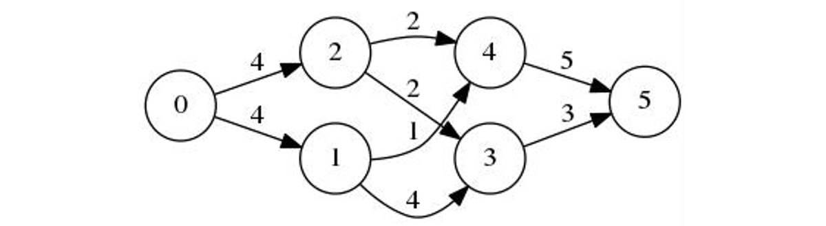
A good comparison of the benefits A* brings over simple SPF may be shown with this picture of pathfinding on a rectangular grid without diagonal connections, where each node is labeled with its 2d-coordinates. To find the path from node (0 0) to (2 2) (length 4) using the Dijkstra’s algorithm, we’ll need to visit all of the points in the grid:
With A*, however, we’ll move straight to the point:
The final path, in these pictures, is selected by the rule to always open the left neighbor first.
Maximum Flow
Weighted directed graphs are often used to represent different kinds of networks. And one of the main tasks on such networks is efficient capacity planning. The main algorithm for that is Maximum Flow calculation. It works on so-called transport networks containing three kinds of vertices: a source, a sink, and intermediate nodes. The source has only outgoing edges, the sink has only incoming, and all the other nodes obey the balance condition: the total weights (flow) of all incoming and outgoing edges are equal. The task of determining maximum flow is to estimate the largest amount that can flow through the whole net from the source to the sink. Besides knowing the actual capacity of the network, it also allows finding the bottlenecks and edges that are not fully utilized. From this point of view, the problem is called Minimum Cut estimation.
There are many approaches to solving this problem. The most direct and intuitive of them is the Ford-Fulkerson method. Once again, it is a greedy algorithm that computes the maximum flow by trying all the paths from source to sink until there is some residual capacity available. These paths are called “augmented paths” as they augment the network flow. And, to track the residual capacity, a copy of the initial weight graph called the “residual graph” is maintained. With each new path added to the total flow, its flow is subtracted from the weights of all of its edges in the residual graph. Besides — and this is the key point in the algorithm that allows it to be optimal despite its greediness — the same amount is added to the backward edges in the residual graph. The backward edges don’t exist in the original graph, and they are added to the residual graph in order to let the subsequent iterations reduce the flow along some edge, but not below zero. Why this restriction may be necessary? Each graph node has a maximum input and output capacity. It is possible to saturate the output capacity by different input edges and the optimal edge to use depends on the whole graph, so, in a single greedy step, it’s not possible to determine over which edges more incoming flow should be directed. The backward edges virtually increase the output capacity by the value of the seized input capacity thus allowing the algorithm to redistribute the flow later on if necessary.
We’ll implement the Ford-Fulkerson Algorithm using the matrix graph representation. First of all, to show it in action, and also as it’s easy to deal with backward edges in a matrix as they are already present, just with zero initial capacity. However, as this matrix will be sparse in the majority of the cases, to achieve optimal efficiency, just like with most other graph algorithms, we’ll need to use a better way to store the edges: for instance, an edge list. With it, we could implement the addition of backward edges directly but lazily during the processing of each augmented path.
(defstruct mf-edge
  beg end capacity)

(defun max-flow (g)
  (let ((rg (copy-array g))  ; residual graph
        (rez 0))
    (loop :for path := (aug-path rg) :while path :do
      (let ((flow most-positive-fixnum))
        ;; the flow along the path is the residual capacity of the thinnest edge
        (dolist (edge path)
          (let ((cap (mf-edge-capacity edge)))
            (when (< (abs cap) flow)
              (setf flow (abs cap)))))
        (dolist (edge path)
          (with-slots (beg end) edge
            (decf (aref rg beg end) flow)
            (incf (aref rg end beg) flow)))
        (incf rez flow)))
    rez))

(defun aug-path (g)
  (rtl:with ((sink (1- (array-dimension g 0)))
             (visited (make-array (1+ sink) :initial-element nil)))
    (labels ((dfs (g i)
               (if (zerop (aref g i sink))
                   (dotimes (j sink)
                     (unless (or (zerop (aref g i j))
                                 (aref visited j))
                       (rtl:when-it (dfs g j)
                         (setf (aref visited j) t)
                         (return (cons (make-mf-edge
                                        :beg i :end j
                                        :capacity (aref g i j))
                                      rtl:it)))))
                   (list (make-mf-edge
                          :beg i :end sink
                          :capacity (aref g i sink))))))
      (dfs g 0))))

CL-USER> (max-flow #2A((0 4 4 0 0 0)
                       (0 0 0 4 2 0)
                       (0 0 0 1 2 0)
                       (0 0 0 0 0 3)
                       (0 0 0 0 0 5))))
7
So, as you can see from the code, to find an augmented path, we need to perform DFS on the graph from the source, sequentially examining the edges with some residual capacity to find a path to the sink.
A peculiarity of this algorithm is that there is no certainty that we’ll eventually reach the state when there will be no augmented paths left. The FFA works correctly for integer and rational weights, but when they are irrational it is not guaranteed to terminate. (The Lisp numeric tower provides the programmer with a chance to use rational-only arithmetic in place of floating point numbers, therefore ensuring algorithm termination). When the capacities are integers, the runtime of Ford-Fulkerson is bounded by O(E f) where f is the maximum flow in the graph. This is because each augmented path can be found in O(E) time and it increases the flow by an integer amount of at least 1. A variation of the Ford-Fulkerson algorithm with guaranteed termination and a runtime independent of the maximum flow value is the Edmonds-Karp algorithm, which runs in O(V E^2).
Graphs in Action: PageRank
Another important set of problems from the field of network analysis is determining “centers of influence”, densely and sparsely populated parts, and “cliques”. PageRank is the well-known algorithm for ranking the nodes in terms of influence (i.e. the number and weight of incoming connections they have), which was the secret sauce behind Google’s initial success as a search engine. It will be the last of the graph algorithms we’ll discuss in this chapter, so many more will remain untouched. We’ll be returning to some of them in the following chapters, and you’ll be seeing them in many problems once you develop an eye for spotting the graphs hidden in many domains.
The PageRank algorithm outputs a probability distribution of the likelihood that a person randomly clicking on links will arrive at any particular page. This distribution ranks the relative importance of all pages. The probability is expressed as a numeric value between 0 and 1, but Google used to multiply it by 10 and round to the greater integer, so PR of 10 corresponded to the probability of 0.9 and more and PR=1 — to the interval from 0 to 0.1. In the context of PageRank, all web pages are the nodes in the so-called webgraph, and the links between them are the edges, originally, weighted equally.
PageRank is an iterative algorithm that may be considered an instance of the very popular, in unsupervised optimization and machine learning, Expectation Maximization (EM) approach. The general idea of EM is to randomly initialize the quantities that we want to estimate, and then iteratively recalculate each quantity, using the information from the neighbors, to “move” it closer to the value that ensures optimality of the target function. Epochs (an iteration that spans the whole data set using each node at most once) of such recalculation should continue either until the whole epoch doesn’t produce a significant change of the loss function we’re optimizing, i.e. we have reached the stationary point, or a satisfactory number of iterations was performed. Sometimes a stationary point either can’t be reached or will take too long to reach, but, according to Pareto’s principle, 20% of effort might have brought us 80% to the goal.
In each epoch, we recalculate the PageRank of all nodes by transferring weights from a node equally to all of its neighbors. The neighbors with more inbound connections will thus receive more weight. However, the PageRank concept adds a condition that an imaginary surfer who is randomly clicking on links will eventually stop clicking. The probability that the transfer will continue is called a damping factor d. Various studies have tested different damping factors, but it is generally assumed that the damping factor for the webgraph will be set around 0.85. The damping factor is subtracted from 1 (and in some variations of the algorithm, the result is divided by the number of documents in the collection) and this term is then added to the product of the damping factor and the sum of the incoming PageRank scores. The damping factor is subtracted from 1 (and in some variations of the algorithm, the result is divided by the number of documents (N) in the collection) and this term is then added to the product of the damping factor and the sum of the incoming PageRank scores. So the PageRank of a page is mostly derived from the PageRanks of other pages. The damping factor adjusts the derived value downward.
Implementation
Actually, PageRank can be computed both iteratively and algebraically. In algebraic form, each PageRank iteration may be expressed simply as:
(setf pr (+ (* d (mat* g pr))
            (/ (- 1 d) n)))
where g is the graph incidence matrix and pr is the vector of PageRank for each node.
However, the definitive property of PageRank is that it is estimated for huge graphs. I.e., directly representing them as matrices isn’t possible, nor is performing the matrix operations on them. The iterative algorithm gives more control, as well as distribution of the computation, so it is usually preferred in practice not only for PageRank but also for most other optimization techniques. So PageRank should be viewed primarily as a distributed algorithm. The need to implement it on a large cluster triggered the development by Google of the influential MapReduce distributed computation framework.
Here is a simplified PageRank implementation of the iterative method:
(defun pagerank (g &key (d 0.85) (repeat 100))
  (rtl:with ((n (length (nodes g)))
             (pr (make-arrray n :initial-element (/ 1 n))))
    (loop :repeat repeat :do
      (let ((pr2 (map 'vector (lambda (x) (- 1 (/ d n)))
                      pr)))
        (dokv (i node nodes)
          (let ((p (aref pr i))
                (m (length (node-children node))))
            (rtl:dokv (j child (node-children node)))
              (incf (aref pr2 j) (* d (/ p m)))))
        (setf pr pr2)))
     pr))
We use the same graph representation as previously and perform the update “backwards”: not by gathering all incoming edges, which will require us to add another layer of data that is both not necessary and hard to maintain, but transferring the PR value over outgoing edges one by one. Such an approach also makes the computation trivial to distribute as we can split the whole graph into arbitrary set of nodes and the computation for each set can be performed in parallel: we’ll just need to maintain a local copy of the pr2 vector and merge it at the end of each iteration by simple summation. This method naturally fits the map-reduce framework that was invented at Google to perform Pagerank and other similar calculations distributed over thousands of machines. The the inner node loop consitutes the essense of the map step, while the reduce step consists in merging of the vectors obtained from each mapper. To see that let’s refactor the above code:
;; this function will be executed by mapper workers
(defun pr1 (node n p &key (d 0.85))
  (let ((pr (make-arrray n :initial-element 0))
        (m (hash-table-count (node-children node))))
    (rtl:dokv (j child (node-children node))
      (setf (aref pr j) (* d (/ p m))))
    pr))

(defun pagerank-mr (g &key (d 0.85) (repeat 100))
  (rtl:with ((n (length (nodes g)))
             (pr (make-arrray n :initial-element (/ 1 n))))
    (loop :repeat repeat :do
      (setf pr (map 'vector (lambda (x)
                              (- 1 (/ d n)))
                    (reduce 'vec+ (map 'vector (lambda (node p)
                                                 (pr1 node n p :d d))
                                       (nodes g)
                                       pr)))))
    pr))
Here, we have used the standard Lisp map and reduce functions, but a map-reduce framework will provide replacement functions which, behind-the-scenes, will orchestrate parallel execution of the provided code. We will talk a bit more about map-reduce and see such framework in the last chapter of this book.
One more thing to note is that the latter approach differs from the original version in that each mapper operates independently on an isolated version of the pr vector, and thus the execution of Pagerank on the subsequent nodes during a single iteration will see an older input value p. However, since the algorithm is stochastic and the order of calculations is not deterministic, this is acceptable: it may impact only the speed of convergence (and hence the number of iterations needed) but not the final result.
Take-Aways
- The more we progress into advanced topics of this book, the more apparent will be the tendency to reuse the approaches, tools, and technologies we have developed previously. Graph algorithms are good demonstrations of new features and qualities that can be obtained by a smart combination and reuse of existing data structures.
- Many graph algorithms are greedy, which means that they use the locally optimal solution trying to arrive at a global one. This phenomenon is conditioned by the structure — or rather lack of structure — of graphs that don’t have a specific hierarchy to guide the optimal solution. The greediness, however, shouldn’t mean suboptimality. In many greedy algorithms, like FFA, there is a way to play back the wrong solution. Others provide a way to trade off execution speed and optimality. A good example of the latter approach is Beam search that has a configurable beam size parameter that allows the programmer to choose speed or optimality of the end result.
- In A, we had a first glimpse of heuristic algorithms — an area that may be quite appealing to many programmers who are used to solving the problem primarily optimizing for its main scenarios. This approach may lack some mathematical rigor, but it also has its place and we’ll see other heuristic algorithms in the following chapters that are, like A, the best practical solution in their domains: for instance, the Monte Carlo Tree Search (MCTS).
- Another thing that becomes more apparent in the progress of this book is how small the percentage of the domain we can cover in detail in each chapter. This is true for graphs: we have just scratched the surface and outlined the main approaches to handling them. We’ll see more of graph-related stuff in the following chapters, as well. Graph algorithms may be quite useful in a great variety of areas that not necessarily have a direct formulation as graph problems (like maps or networks do) and so developing an intuition to recognize the hidden graph structure may help the programmer reuse the existing elegant techniques instead of having to deal with own cumbersome ad-hoc solutions.