6 Linked Lists
Linked data structures are in many ways the opposite of the contiguous ones that we have explored to some extent in the previous chapter using the example of arrays. In terms of complexity, they fail where those ones shine (first of all, at random access) — but prevail at scenarios when a repeated modification is necessary. In general, they are much more flexible and so allow the programmer to represent almost any kind of a data structure, although the ones that require such level of flexibility may not be too frequent. Usually, they are specialized trees or graphs.
The basic linked data structure is a singly-linked list.
Just like arrays, lists in Lisp may be created both with a literal syntax for constants and by calling a function — make-list — that creates a list of a certain size filled with nil elements. Besides, there’s a handy list utility that is used to create lists with the specified content (the analog of rtl:vec).
CL-USER> '("hello" world 111)
("hello" WORLD 111)
CL-USER> (make-list 3)
(NIL NIL NIL)
CL-USER> (list "hello" 'world 111)
("hello" WORLD 111)
An empty list is represented as () and, interestingly, in Lisp, it is also a synonym of logical falsehood (nil). This property is used very often, and we’ll have a chance to see that.
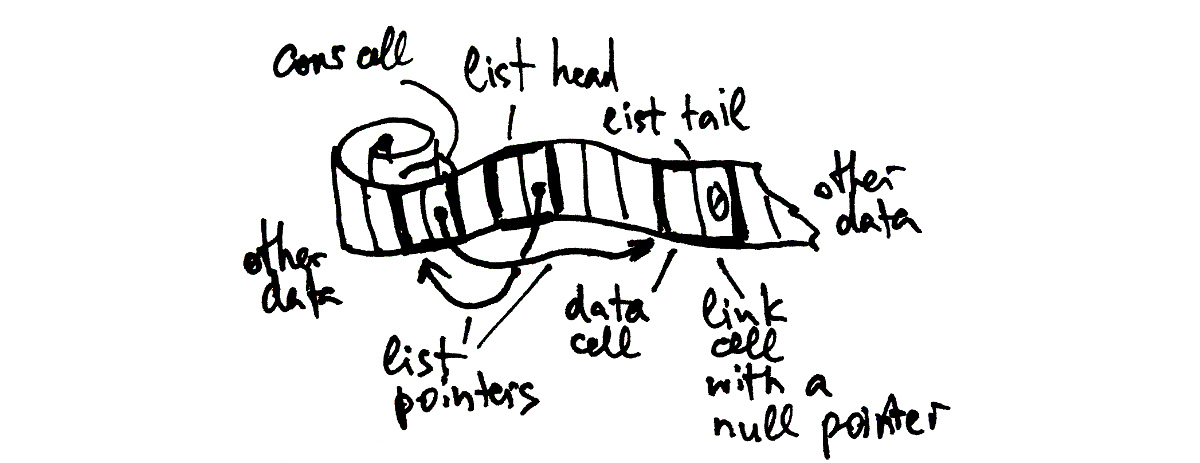
If we were to introduce our own lists, which may be quite a common scenario in case the built-in ones’ capabilities do not suit us, we’d need to define the structure “node”, and our list would be built as a chain of such nodes. We might have wanted to store the list head and, possibly, tail, as well as other properties like size. All in all, it would look like the following:
(defstruct list-cell
  data
  next)

(defstruct our-own-list
  (head nil :type (or list-cell null))
  (tail nil :type (or list-cell null)))

CL-USER> (let ((tail (make-list-cell :data "world")))
           (make-our-own-list
            :head (make-list-cell
                   :data "hello"
                   :next tail)
            :tail tail))
#S(OUR-OWN-LIST
   :HEAD #S(LIST-CELL
            :DATA "hello"
            :NEXT #S(LIST-CELL :DATA "world" :NEXT NIL))
   :TAIL #S(LIST-CELL :DATA "world" :NEXT NIL))
Lists as Sequences
Alongside arrays, list is the other basic data structure that implements the sequence abstract data type. Let’s consider the complexity of basic sequence operations for linked lists:
- so-called random access, i.e. access by index of a random element, requires
O(n)time as we have to traverse all the preceding elements before we can reach the desired one (n/2operations on average) - yet, once we have reached some element, removing it or inserting something after it takes
O(1) - subsequencing is also
O(n)
Getting the list length, in the basic case, is also O(n) i.e. it requires full list traversal. It is possible, though, to store list length as a separate slot, tracking each change on the fly, which means O(1) complexity. Lisp, however, implements the simplest variant of lists without size tracking. This is an example of a small but important decision that real-world programming is full of. Why is such a solution the right thing™, in this case? Adding the size counter to each list would have certainly made this common length operation more effective, but the cost of doing that would’ve included: increase in occupied storage space for all lists, a need to update size in all list modification operations, and, possibly, a need for a more complex cons cell implementation.1 These considerations make the situation with lists almost opposite to arrays, for which size tracking is quite reasonable because they change much less often and not tracking the length historically proved to be a terrible security decision. So, what side to choose? A default approach is to prefer the solution which doesn’t completely rule out the alternative strategy. If we were to choose a simple cons-cell sans size (what the authors of Lisp did) we’ll always be able to add the “smart” list data structure with the size field, on top of it. Yet, stripping the size field from built-in lists won’t be possible. Similar reasoning is also applicable to other questions, such as: why aren’t lists, in Lisp, doubly-linked. Also, it helps that there’s no security implication as lists aren’t used as data exchange buffers, for which the problem manifests itself.
For demonstration, let’s add the size field to our-own-list (and, meanwhile, consider all the functions that will need to update it…):
(defstruct our-own-list
  (head nil :type (or list-cell null))
  (tail nil :type (or list-cell null))
  (size 0 :type (integer 0)))
Given that obtaining the length of a list, in Lisp, is an expensive operation, a common pattern in programs that require multiple requests of the length field is to store its value in some variable at the beginning of the algorithm and then use this cached value, updating it if necessary.
As we see, lists are quite inefficient in random access scenarios. However, many sequences don’t require random access and can satisfy all the requirements of a particular use case using just the sequential one. That’s one of the reasons why they are called sequences, after all. And if we consider the special case of list operations at index 0 they are, obviously, efficient: both access and addition/removal is O(1). Also, if the algorithm requires a sequential scan, list traversal is rather efficient too. Yet, it is not as good as array traversal for it still requires jumping over the memory pointers. There are numerous sequence operations that are based on sequential scans. The most common is map, which we analyzed in the previous chapter. It is the functional programming alternative to looping, a more high-level operation, and thus simpler to understand for the common cases, although less versatile.
map is a function that works with different types of built-in sequences. It takes as the first argument the target sequence type (if nil is supplied it won’t create the resulting sequence and so will be used just for side-effects). Here is a polymorphic example involving lists and vectors:
CL-USER> (map 'vector '+
              '(1 2 3 4 5)
              #(1 2 3))
#(2 4 6)
map applies the function provided as its second argument (here, addition) sequentially to every element of the sequences that are supplied as other arguments, until one of them ends, and records the result in the output sequence. map would have been even more intuitive, if it just had used the type of the first argument for the result sequence, i.e. be a “do what I mean” dwim-map, while a separate advanced variant with result-type selection might have been used in the background. Unfortunately, the current standard scheme is not for change, but we can define our own wrapper function:
(defun dwim-map (fn seq &rest seqs)
  "A thin wrapper over MAP that uses the type of the first SEQ for the result."
  (apply 'map (type-of seq) fn seqs))
Historically, map in Lisp was originally used for lists in its list-specific variants that predated the generic map. Most of those functions like mapcar, mapc, and mapcan (replaced in RUTILS by a safer flat-map) are still widely used today.
Now, let’s see a couple of examples of using mapping. Suppose that we’d like to extract odd numbers from a list of numbers. Using mapcar as a list-specific map we might try to call it with an anonymous function that tests its argument for oddity and keeps them in such case:
CL-USER> (mapcar (lambda (x) (when (oddp x) x))
                 (rtl:range 1 10))
(1 NIL 3 NIL 5 NIL 7 NIL 9)
However, the problem is that non-odd numbers still have their place reserved in the result list, although it is not filled by them. Keeping only the results that satisfy (or don’t) certain criteria and discarding the others is a very common pattern that is known as “filtering”. There’s a set of Lisp functions for such scenarios: remove, remove-if, and remove-if-not, as well as RUTILS’ complements to them keep-if and keep-if-not. We can achieve the desired result adding remove to the picture:
CL-USER> (remove nil (mapcar (lambda (x) (when (oddp x) x))
                             (rtl:range 1 10)))
(1 3 5 7 9)
A more elegant solution will use the remove-if(-not) or rtl:keep-if(-not) variants. remove-if-not is the most popular among these functions. It takes a predicate and a sequence and returns the sequence of the same type holding only the elements that satisfy the predicate:
CL-USER> (remove-if-not 'oddp (range 1 10))
(1 3 5 7 9)
Using such high-level mapping functions is very convenient, which is why there’s a number of other -if(-not) operations, like find(-if(-not)), member(-if(-not)), position(-if(-not)), etc.
The implementation of mapcar or any other list mapping function, including your own task-specific variants, follows the same pattern of traversing the list accumulating the result into another list and reversing it, in the end:
(defun simple-mapcar (fn list)
  (let ((rez (list)))
    (dolist (item list)
      (setf rez (cons (funcall fn item) rez)))
    (reverse rez)))
The function cons is used to add an item to the beginning of the list. It creates a new list head that points to the previous list as its tail.
From the complexity point of view, if we compare such iteration with looping over an array we’ll see that it is also a linear traversal that requires twice as many operations as with arrays because we need to traverse the result fully once again, in the end, to reverse it. Its advantage, though, is higher versatility: if we don’t know the size of the resulting sequence (for example, in the case of remove-if-not) we don’t have to change anything in this scheme and just add a filter line ((when (oddp item) ...), while for arrays we’d either need to use a dynamic array (that will need constant resizing and so have at least the same double number of operations) or pre-allocate the full-sized result sequence and then downsize it to fit the actual accumulated number of elements, which may be problematic when we deal with large arrays.
Lists as Functional Data Structures
The distinction between arrays and linked lists in many ways reflects the distinction between the imperative and functional programming paradigms. Within the imperative or, in this context, procedural approach, the program is built out of low-level blocks (conditionals, loops, and sequentials) that allow for the most fine-tuned and efficient implementation, at the expense of abstraction level and modularization capabilities. It also heavily utilizes in-place modification and manual resource management to keep overhead at a minimum. An array is the most suitable data-structure for such a way of programming. Functional programming, on the contrary, strives to bring the abstraction level higher, which may come at a cost of sacrificing efficiency (only when necessary, and, ideally, only for non-critical parts). Functional programs are built by combining referentially transparent computational procedures (aka “pure functions”) that operate on more advanced data structures (either persistent ones or having special access semantics, e.g. transactional) that are also more expensive to manage but provide additional benefits.
Singly-linked lists are a simple example of functional data structures. A functional or persistent data structure is the one that doesn’t allow in-place modification. In other words, to alter the contents of the structure a fresh copy with the desired changes should be created. The flexibility of linked data structures makes them suitable for serving as functional ones. We have seen the cons operation that is one of the earliest examples of non-destructive, i.e. functional, modification. This action prepends an element to the head of a list, and as we’re dealing with the singly-linked list the original doesn’t have to be updated: a new cons cell is added in front of it with its next pointer referencing the original list that becomes the new tail. This way, we can preserve both the pointer to the original head and add a new head. Such an approach is the basis for most of the functional data structures: the functional trees, for example, add a new head and a new route from the head to the newly added element, adding new nodes along the way — according to the same principle.
It is interesting, though, that lists can be used in destructive and non-destructive fashion likewise. There are both low- and high-level functions in Lisp that perform list modification, and their existence is justified by the use cases in many algorithms. Purely functional lists render many of the efficient list algorithms useless. One of the high-level list modification function is nconc. It concatenates two lists together updating in the process the next pointer of the last cons cell of the first list:
CL-USER> (let ((l1 (list 1 2 3))
               (l2 (list 4 5 6)))
           (nconc l1 l2)  ; note no assignment to l1
           l1)            ; but it is still changed
(1 2 3 4 5 6)
There’s a functional variant of this operation, append, and, in general, it is considered distasteful to use nconc as the risk of unwarranted modification outweights the minor efficiency gains. Using append we’ll need to modify the previous piece of code because otherwise the newly created list will be garbage-collected immediately:
CL-USER> (let ((l1 (list 1 2 3))
               (l2 (list 4 5 6)))
           (setf l1 (append l1 l2))
           l1)
(1 2 3 4 5 6)
The low-level list modification operations are rplaca and rplacd. They can be combined with list-specific accessors nth and nthcdr that provide indexed access to list elements and tails respectively. Here’s, for example, how to add an element in the middle of a list:
CL-USER> (let ((l1 (list 1 2 3)))
           (rplacd (nthcdr 0 l1)
                   (cons 4 (nthcdr 1 l1)))
           l1)
(1 4 2 3)
Just to re-iterate, although functional list operations are the default choice, for efficient implementation of some algorithms, you’ll need to resort to the ugly destructive ones.
Different Kinds of Lists
We have, thus far, seen the most basic linked list variant — a singly-linked one. It has a number of limitations: for instance, it’s impossible to traverse it from the end to the beginning. Yet, there are many algorithms that require accessing the list from both sides or do other things with it that are inefficient or even impossible with the singly-linked one, hence other, more advanced, list variants exist.
But first, let’s consider an interesting tweak to the regular singly-linked list — a circular list. It can be created from the normal one by making the last cons cell point to the first. It may seem like a problematic data structure to work with, but all the potential issues with infinite looping while traversing it are solved if we keep a pointer to any node and stop iteration when we encounter this node for the second time. What’s the use for such structure? Well, not so many, but there’s a prominent one: the ring buffer. A ring or circular buffer is a structure that can hold a predefined number of items and each item is added to the next slot of the current item. This way, when the buffer is completely filled it will wrap around to the first element, which will be overwritten at the next modification. By our buffer-filling algorithm, the element to be overwritten is the one that was written the earliest for the current item set. Using a circular linked list is one of the simplest ways to implement such a buffer. Another approach would be to use an array of a certain size moving the pointer to the next item by incrementing an index into the array. Obviously, when the index reaches array size it should be reset to zero.
A more advanced list variant is a doubly-linked one, in which all the elements have both the next and previous pointers. The following definition, using inheritance, extends our original list-cell with a pointer to the previous element. Thanks to the basic object-oriented capabilities of structs, it will work with the current definition of our-own-list as well, and allow it to function as a doubly-linked list.
(defstruct (list-cell2 (:include list-cell))
  prev)
Yet, we still haven’t shown the implementation of the higher-level operations of adding and removing an element to/from our-own-list. Obviously, they will differ for singly- and doubly-linked lists, and that distinction will require us to differentiate the doubly-linked list types. That, in turn, will demand invocation of a rather heavy OO-machinery, which is beyond the subject of this book. Instead, for now, let’s just examine the basic list addition function, for the doubly-linked list:
(defun our-cons2 (data list)
  (when (null list) (setf list (make-our-own-list)))
  (let ((new-head (make-list-cell2
                   :data data
                   :next @list.head)))
    (when (rtl:? list 'head)
      (setf (rtl:? list 'head 'prev) new-head))
    (make-our-own-list
     :head new-head
     :tail (rtl:? list 'tail)
     :size (1+ (rtl:? list 'size)))))
The first thing to note is the use of the @ syntactic sugar, from RUTILS, that implements the mainstream dot notation for slot-value access (i.e. @list.head.prev refers to the prev field of the head field of the provided list structure of the assumed our-own-list type, which in a more classically Lispy, although cumbersome, variants may look like one of the following: (our-cons2-prev (our-own-list-head list)) or (slot-value (slot-value list 'head) 'prev).2
More important here is that, unlike for the singly-linked list, this function requires an in-place modification of the head element of the original list: setting its prev pointer. Immediately making doubly-linked lists non-persistent.
Finally, the first line is the protection against trying to access the null list (that will result in a much-feared, especially in Java-land, null-pointer exception class of error).
At first sight, it may seem that doubly-linked lists are more useful than singly-linked ones. But they also have higher overhead so, in practice, they are used quite sporadically. We may see just a couple of use cases on the pages of this book. One of them is presented in the next part — a double-ended queue.
Besides doubly-linked, there are also association lists that serve as a variant of key-value data structures. At least 3 types may be found in Common Lisp code, and we’ll briefly discuss them in the chapter on key-value structures. Finally, a skip list is a probabilistic data structure based on singly-linked lists, that allows for faster search, which we’ll also discuss in a separate chapter on probabilistic structures. Other more esoteric list variants, such as self-organized list and XOR-list, may also be found in the literature — but very rarely, in practice.
FIFO & LIFO
The flexibility of lists allows them to serve as a common choice for implementing a number of popular abstract data structures.
Queue
A queue or FIFO has the following interface:
-
enqueuean item at the end -
dequeuethe first element: get it and remove it from the queue
It imposes a first-in-first-out (FIFO) ordering on the elements. A queue can be implemented directly with a singly-linked list like our-own-list. Obviously, it can also be built on top of a dynamic array but will require permanent expansion and contraction of the collection, which, as we already know, isn’t the preferred scenario for their usage.
There are numerous uses for the queue structures for processing items in a certain order (some of which we’ll see in further chapters of this book).
Stack
A stack or LIFO (last-in-first-out) is even simpler than a queue, and it is used even more widely. Its interface is:
-
pushan item on top of the stack making it the first element -
popan item from the top: get it and remove it from the stack
A simple Lisp list can serve as a stack, and you can see such uses in almost every file with Lisp code. The most common pattern is result accumulation during iteration: using the stack interface, we can rewrite simple-mapcar in an even simpler way (which is idiomatic Lisp):
(defun simple-mapcar (fn list)
  (let ((rez (list)))
    (dolist (item list)
      (push (funcall fn item) rez))
    (reverse rez)))
Stacks hold elements in reverse-chronological order and can thus be used to keep the history of changes to be able to undo them. This feature is used in procedure calling conventions by the compilers: there exists a separate segment of program memory called the Stack segment, and when a function call happens (beginning from the program’s entry point called the main function in C) all of its arguments and local variables are put on this stack as well as the return address in the program code segment where the call was initiated. Such an approach allows for the existence of local variables that last only for the duration of the call and are referenced relative to the current stack head and not bound to some absolute position in memory like the global ones. After the procedure call returns, the stack is “unwound” and all the local data is forgotten returning the context to the same state in which it was before the call. Such stack-based history-keeping is a very common and useful pattern that may be utilized in userland code likewise.
Lisp itself also uses this trick to implement global variables with a capability to have context-dependent values through the extent of let blocks: each such variable also has a stack of values associated with it. This is one of the most underappreciated features of the Lisp language used quite often by experienced lispers. Here is a small example with a standard global variable (they are called special in Lisp parlance due to this special property) *standard-output* that stores a reference to the current output stream:
CL-USER> (print 1)
1
1
CL-USER> (let ((*standard-output* (make-broadcast-stream)))
           (print 1))
1
In the first call to print, we see both the printed value and the returned one, while in the second — only the return value of the print function, while it’s output is sent, effectively, to /dev/null.
Stacks can be also used to implement queues. We’ll need two of them to do that: one will be used for enqueuing the items and the other — for dequeuing. Here’s the implementation:
(defstruct queue
  head
  tail)

(defun enqueue (item queue)
  (push item (rtl:? queue 'head)))

(defun dequeue (queue)
  ;; Here and in the next condition, we use the property that an empty list
  ;; is also logically false. This is discouraged by many Lisp style-guides,
  ;; but in many cases such code is not only more compact but also more clear.
  (unless @queue.tail
    (do ()
        ;; this loop continues until the head becomes empty
        ((null (rtl:? queue 'head)))
      (push (pop (rtl:? queue 'head)) (rtl:? queue 'tail))))
      ;; By pushing all the items from the head to the tail,
      ;; we reverse their order — this is the second reversing
      ;; that cancels the reversing performed when we push the items
      ;; onto the head, so it restores the original order.
  (when (rtl:? queue 'tail)
    (values (pop (rtl:? queue 'tail))
            t)))  ; this second value is used to indicate
                  ; that the queue was not empty

CL-USER> (let ((q (make-queue)))
           (print q)
           (enqueue 1 q)
           (enqueue 2 q)
           (enqueue 3 q)
           (print q)
           (dequeue q)
           (print q)
           (enqueue 4 q)
           (print q)
           (dequeue q)
           (print q)
           (dequeue q)
           (print q)
           (dequeue q)
           (print q)
           (dequeue q))
#S(QUEUE :HEAD NIL :TAIL NIL)
#S(QUEUE :HEAD (3 2 1) :TAIL NIL)
#S(QUEUE :HEAD NIL :TAIL (2 3))
#S(QUEUE :HEAD (4) :TAIL (2 3))
#S(QUEUE :HEAD (4) :TAIL (3))
#S(QUEUE :HEAD (4) :TAIL NIL)
#S(QUEUE :HEAD NIL :TAIL NIL)
NIL  ; no second value indicates that the queue is now empty
Such queue implementation still has O(1) operation times for enqueue/dequeue. Each element will experience exactly 4 operations: 2 pushs and 2 pops (for the head and tail). Though, for dequeue this will be the average (amortized) performance, while there may be occasional peaks in individual operation runtimes: specifically, after long uninterrupted series of enqueues.
Another stack-based structure is the stack with a minimum element, i.e. some structure that not only holds elements in LIFO order but also keeps track of the minimum among them. The challenge is that if we just add the min slot that holds the current minimum, when this minimum is popped out of the stack we’ll need to examine all the remaining elements to find the new minimum. We can avoid this additional work by adding another stack — a stack of minimums. Now, each push and pop operation requires us to also check the head of this second stack and, in case the added/removed element is the minimum, push it to the stack of minimums or pop it from there, accordingly.
A well-known algorithm that illustrates stack usage is fully-parenthesized arithmetic expressions evaluation:
(defun arith-eval (expr)
  "EXPR is a list of symbols that may include:
   square brackets, arithmetic operations, and numbers."
  (let ((ops ())
        (vals ())
        (op nil)
        (val nil))
    (dolist (item expr)
      (case item
        ([ ) ; do nothing
        ((+ - * /) (push item ops))
        (] (setf op (pop ops)
                 val (pop vals))
           (case op
             (+ (incf val (pop vals)))
             (- (decf val (pop vals)))
             (* (setf val (* val (pop vals))))
             (/ (setf val (/ val (pop vals)))))
           (push val vals))
        (otherwise (push item vals))))
    (pop vals)))

CL-USER> (arith-eval '([ 1 + [ [ 2 + 3 ] * [ 4 * 5 ] ] ] ]))
101
Deque
A deque is a short name for a double-ended queue, which can be traversed in both orders: FIFO and LIFO. It has 4 operations: push-front and push-back (also called shift), pop-front and pop-back (unshift). This structure may be implemented with a doubly-linked list or likewise a simple queue with 2 stacks. The difference for the 2-stacks implementation is that now items may be pushed back and forth between head and tail depending on the direction we’re popping from, which results in worst-case linear complexity of such operations: when there’s constant alteration of front and back directions.
The use case for such structure is the algorithm that utilizes both direct and reverse ordering: a classic example being job-stealing algorithms, when the main worker is processing the queue from the front, while other workers, when idle, may steal the lowest priority items from the back (to minimize the chance of a conflict for the same job).
Stacks in Action: SAX Parsing
Custom XML parsing is a common task for those who deal with different datasets, as many of them come in XML form, for example, Wikipedia and other Wikidata resources. There are two main approaches to XML parsing:
- DOM parsing reads the whole document and creates its tree representation in memory. This technique is handy for small documents, but, for huge ones, such as the dump of Wikipedia, it will quickly fill all available memory. Also, dealing with the deep tree structure, if you want to extract only some specific pieces from it, is not very convenient.
- SAX parsing is an alternative variant that uses the stream approach. The parser reads the document and, upon completing the processing of a particular part, invokes the relevant callback: what to do when an open tag is read, when a closed one, and with the contents of the current element. These actions happen for each tag, and we can think of the whole process as traversing the document tree utilizing the so-called “visitor pattern”: when visiting each node we have a chance to react after the beginning, in the middle, and in the end.
Once you get used to SAX parsing, due to its simplicity, it becomes a tool of choice for processing XML, as well as JSON and other formats that allow for a similar stream parsing approach. Often the simplest parsing pattern is enough: remember the tag we’re looking at, and when it matches a set of interesting tags, process its contents. However, sometimes, we need to make decisions based on the broader context. For example, let’s say, we have the text marked up into paragraphs, which are split into sentences, which are, in turn, tokenized. To process such a three-level structure, with SAX parsing, we could use the following outline (utilizing the primitives from CXML library):
(defclass text-sax (sax:sax-parser-mixin)
  ((parags :initform (list) :accessor sax-parags)
   (parag :initform (list) :accessor sax-parag)
   (sent :initform (list) :accessor sax-sent)
   (tag-stack :initform (list) :accessor sax-tag-stack)))

(defmethod sax:start-element ((sax text-sax)
                              namespace-uri local-name qname attrs)
  (declare (ignore namespace-uri qname attrs))
  (push (rtl:mkeyw local-name) (sax-tag-stack sax)))

(defmethod sax:end-element ((sax text-sax)
                            namespace-uri local-name qname)
  (declare (ignore namespace-uri qname))
  (with-slots (tag-stack sent parag parags) sax
    (case (pop tag-stack)
      (:paragraph (push (reverse parag) parags)
                  (setf parag nil))
      (:sentence (push (reverse sent) parag)
                 (setf sent nil)))))

(defmethod sax:characters ((sax text-sax) text)
  (when (eql :token (first (sax-tag-stack sax)))
    (push text (sax-sent sax))))

(defmethod sax:end-document ((sax text-sax))
  (reverse (sax-parags sax)))
It is our first encounter with the Common Lisp Object System (CLOS) that is based on the concepts of objects pertaining to certain classes and methods specialized on those classes. Objects are, basically, enhanced structs (with multiple inheritance capabilities), while methods allow the programmer to arrange overloaded behavior of the same operations (called “egenric functions” in Lisp parlance) for different classes of inputs into separate self-contained code blocks. CLOS is a very substantial topic that is beyond the scope of this book3. Yet, for those familiar with the OOP paradigm and its implementation in any programming language, the idea behind the above code should be familiar. In fact, this is how SAX parsing is handled in similar Python or Java libraries: by extending the provided base class and implementing the specialized versions of its API functions.
This code returns the accumulated structure of paragraphs from the sax:end-document method. It uses two stacks — for the current sentence and the current paragraph — to accumulate intermediate data during the parsing process. In a similar fashion, another stack of encountered tags might have been used to exactly track our position in the document tree if there were such necessity. Overall, the more you’ll be using SAX parsing, the more you’ll realize that stacks are enough to address 99% of the arising challenges.
Here is an example of running the parser on a toy XML document:
CL-USER> (cxml:parse-octets
          ;; FLEXI-STREAMS library is used here
          (flex:string-to-octets "<text>
  <paragraph>
    <sentence><token>A</token><token>test</token></sentence>
    <sentence><token>foo</token><token>bar</token><token>baz</token></sentence>
  </paragraph>
  <paragraph>
    <sentence><token>42</token></sentence>
  </paragraph>
</text>")
           (make-instance 'text-sax))
((("A" "test")
  ("foo" "bar" "baz"))
 (("42")))
Lists as Sets
Another very important abstract data structure is a Set. It is a collection that holds each element only once no matter how many times we add it there. This structure may be used in a variety of cases: when we need to track the items we have already seen and processed, when we want to calculate some relations between groups of elements, and so forth.
Basically, its interface consists of set-theoretic operations:
- add/remove an item
- check whether an item is in the set
- check whether a set is a subset of another set
- union, intersection, difference, etc.
Sets have an interesting aspect that an efficient implementation of element-wise operations (add/remove/member) and set-wise (union/…) require the use of different concrete data-structures, so a choice should be made depending on the main use case. One way to implement sets is by using linked lists. Lisp has standard library support for this with the following functions:
-
adjointo add an item to the list if it’s not already there -
memberto check for item presence in the set -
subsetpfor subset relationship query -
union,intersection,set-difference, andset-exclusive-orfor set operations
This approach works well for small sets (up to tens of elements), but it is rather inefficient, in general. Adding an item to the set or checking for membership will require O(n) operations, while, in the hash-set (that we’ll discuss in the chapter on key-value structures), these are O(1) operations. A naive implementation of union and other set-theoretic operations will require O(n^2) as we’ll have to compare each element from one set with each one from the other. However, if our set lists are in sorted order set-theoretic operations can be implemented efficiently in just O(n) where n is the total number of elements in all sets, by performing a single linear scan over each set in parallel. Using a hash-set will also result in the same complexity.
Here is a simplified implementation of union for sets of numbers built on sorted lists:
(defun sorted-union (s1 s2)
  (let ((rez ()))
    (do ()
        ((and (null s1) (null s2)))
      (let ((i1 (first s1))
            (i2 (first s2)))
        (cond ((null i1) (dolist (i2 s2)
                           (push i2 rez))
                         (return))
              ((null i2) (dolist (i1 s1)
                           (push i1 rez))
                         (return))
              ((= i1 i2) (push i1 rez)
                         (setf s1 (rest s1)
                               s2 (rest s2)))
              ((< i1 i2) (push i1 rez)
                         (setf s1 (rest s1)))
              ;; just T may be used instead
              ;; of the following condition
              ((> i1 i2) (push i2 rez)
                         (setf s2 (rest s2))))))
    (reverse rez)))

CL-USER> (sorted-union '(1 2 3)
                       '(0 1 5 6))
(0 1 2 3 5 6)
This approach may be useful even for unsorted list-based sets as sorting is a merely O(n * log n) operation. Even better though, when the use case requires primarily set-theoretic operations on our sets and the number of changes/membership queries is comparatively low, the most efficient technique may be to keep the lists sorted at all times.
Merge Sort
Speaking about sorting, the algorithms we discussed for array sorting in the previous chapter do not work as efficient for lists for they are based on swap operations, which are O(n), in the list case. Thus, another approach is required, and there exist a number of efficient list sorting algorithms, the most prominent of which is Merge sort. It works by splitting the list into two equal parts until we get to trivial one-element lists and then merging the sorted lists into the bigger sorted ones. The merging procedure for sorted lists is efficient as we’ve seen in the previous example. A nice feature of such an approach is its stability, i.e. preservation of the original order of the equal elements, given the proper implementation of the merge procedure.
(defun merge-sort (list comp)
  (if (null (rest list))
      list
      (let ((half (floor (length list) 2)))
        (merge-lists (merge-sort (subseq seq 0 half) comp)
                     (merge-sort (subseq seq half) comp)
                     comp))))

(defun merge-lists (l1 l2 comp)
  (let ((rez ()))
    (do ()
        ((and (null l1) (null l2)))
      (let ((i1 (first l1))
            (i2 (first l2)))
        (cond ((null i1) (dolist (i l2)
                           (push i rez))
                         (return))
              ((null i2) (dolist (i l1)
                           (push i rez))
                         (return))
              ((funcall comp i1 i2) (push i1 rez)
                                    (setf l1 (rest l1)))
              (t (push i2 rez)
                 (setf l2 (rest l2))))))
    (reverse rez)))
The same complexity analysis as for binary search applies to this algorithm. At each level of the recursion tree, we perform O(n) operations: each element is pushed into the resulting list once, reversed once, and there are at most 4 comparison operations: 3 null checks and 1 call of the comp function. We also need to perform one copy per element in the subseq operation and take the length of the list (although it can be memorized and passed down as the function call argument) on the recursive descent. This totals to not more than 10 operations per element, which is a constant. And the height of the tree is, as we already know, (log n 2). So, the total complexity is O(n * log n).
Let’s now measure the real time needed for such sorting, and let’s compare it to the time of prod-sort (with optimal array accessors) from the Arrays chapter:
Interestingly enough, Merge sort turned out to be around 5 times faster, although it seems that the number of operations required at each level of recursion is at least 2-3 times bigger than for quicksort. Why we got such result is left as an exercise to the reader: I’d start from profiling the function calls and looking where most of the time is wasted…
It should be apparent that the merge-lists procedure works in a similar way to set-theoretic operations on sorted lists that we’ve discussed in the previous part. It is, in fact, provided in the Lisp standard library. Using the standard merge, Merge sort may be written in a completely functional and also generic way to support any kind of sequences:
(defun merge-sort (seq comp)
  (if (or (null seq)  ; avoid expensive length calculation
          (<= (length seq) 1))
      seq
      (let ((half (floor (length seq) 2)))
        (merge (type-of seq)
               (merge-sort (subseq seq 0 half) comp)
               (merge-sort (subseq seq half) comp)
               comp))))
There’s still one substantial difference of Merge sort from the array sorting functions: it is not in-place. So it also requires the O(n * log n) additional space to hold the half sublists that are produced at each iteration. Sorting and merging them in-place is not possible. There are ways to somewhat reduce this extra space usage but not totally eliminate it.
Parallelization of Merge Sort
The extra-space drawback of Merge sort may, however, turn irrelevant if we consider the problem of parallelizing this procedure. The general idea of parallelized implementation of any algorithm is to split the work in a way that allows reducing the runtime proportional to the number of workers performing those jobs. In the ideal case, if we have m workers and are able to spread the work evenly the running time should be reduced by a factor of m. For the Merge sort, it will mean just O(n/m * log n). Such ideal reduction is not always achievable, though, because often there are bottlenecks in the algorithm that require all or some workers to wait for one of them to complete its job.
Here’s a trivial parallel Merge sort implementation that uses the eager-future2 library, which adds high-level data parallelism capabilities based on the Lisp implementation’s multithreading facilities:
(defun parallel-merge-sort (seq comp)
  (if (or (null seq) (<= (length seq) 1))
      seq
      (rtl:with ((half (floor (length seq) 2))
                 (thread1 (eager-future2:pexec
                            (merge-sort (subseq seq 0 half) comp)))
                 (thread2 (eager-future2:pexec
                            (merge-sort (subseq seq half) comp))))
        (merge (type-of seq)
               (eager-future2:yield thread1)
               (eager-future2:yield thread2)
               comp))))
The eager-future2:pexec procedure submits each merge-sort to the thread pool that manages multiple CPU threads available in the system and continues program execution not waiting for it to return. While eager-future2:yield pauses execution until the thread performing the appropriate merge-sort returns.
When I ran our testing function with both serial and parallel merge sorts on my machine, with 4 CPUs, I got the following result:
A speedup of approximately 2x, which is also reflected by the rise in CPU utilization from around 100% (i.e. 1 CPU) to 250%. These are correct numbers as the merge procedure is still executed serially and remains the bottleneck. There are more sophisticated ways to achieve optimal m times speedup, in Merge sort parallelization, but we won’t discuss them here due to their complexity.
Lists and Lisp
Historically, Lisp’s name originated as an abbreviation of “List Processing”, which points both to the significance that lists played in the language’s early development and also to the fact that flexibility (a major feature of lists) was always a cornerstone of its design. Why are lists important to Lisp? Maybe, originally, it was connected with the availability and the good support of this data structure in the language itself. But, quickly, the focus shifted to the fact that, unlike other languages, Lisp code is input in the compiler not in a custom string-based format but in the form of nested lists that directly represent the syntax tree. Coupled with superior support for the list data structure, it opens numerous possibilities for programmatic processing of the code itself, which are manifest in the macro system, code walkers and generators, etc. So, “List Processing” turns out to be not about lists of data, but about lists of code, which perfectly describes the main distinctive feature of this language…
Take-Aways
In this chapter, we have seen the possibilities that the flexibility of linked structures opens: lists were used as sequences, sets, stacks, and queues. We’ll continue utilizing this flexibility over and over in the following parts.
behind-the-scenes# Key-Values
To conclude the description of essential data structures, we need to discuss key-values (kvs), which are the broadest family of structures one can imagine. Unlike arrays and lists, kvs are not concrete structures. In fact, they span, at least in some capacity, all of the popular concrete ones, as well as some obscure.
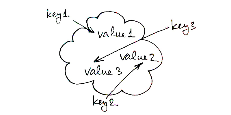
The main feature of kvs is efficient access to the values by some kind of keys that they are associated with. In other words, each element of such data structure is a key-value pair that can be easily retrieved if we know the key, and, on the other hand, if we ask for the key that is not in the structure, the null result is also returned efficiently. By “efficiently”, we usually mean O(1) or, at least, something sublinear (like O(log n)), although, for some cases, even O(n) retrieval time may be acceptable. See how broad this is! So, a lot of different structures may play the role of key-values.
By the way, there isn’t even a single widely-adopted name for such structures. Besides key-values — which isn’t such a popular term (I derived it from key-value stores) — in different languages, they are called maps, dictionaries, associative arrays, tables, objects and so on.
In a sense, these are the most basic and essential data structures. They are so essential that some dynamic languages — for example, Lua, explicitly, and JavaScript, without a lot of advertisement — rely on them as the core (sometimes sole) language’s data structure. Moreover, key-values are used almost everywhere. Below is a list of some of the most popular scenarios:
- implementation of the object system in programming languages
- most of the key-value stores are, for the most part, glorified key-value structures
- internal tables in the operating system (running process table or file descriptor tables in the Linux kernel), programming language environment or application software
- all kinds of memoization and caching
- efficient implementation of sets
- ad hoc or predefined records for returning aggregated data from function calls
- representing various dictionaries (in language processing and beyond)
Considering such a wide spread, it may be surprising that, historically, the programming language community only gradually realized the usefulness of key-values. For instance, such languages as C and C++ don’t have the built-in support for general kvs (if we don’t count structs and arrays, which may be considered significantly limited versions). Lisp, on the contrary, was to some extent pioneering their recognition with the concepts of alists and plists, as well as being one of the first languages to have hash-table support in the standard.
Concrete Key-values
Let’s see what concrete structures can be considered key-values and in which cases it makes sense to use them.
Simple Arrays
Simple sequences, especially arrays, may be regarded as a particular variant of kvs that allows only numeric keys with efficient (and fastest) constant-time access. This restriction is serious. However, as we’ll see below, it can often be worked around with clever algorithms. As a result, arrays actually play a major role in the key-value space, but not in the most straightforward form. Although, if it is possible to be content with numeric keys and their number is known beforehand, vanilla arrays are the best possible implementation option. Example: OS kernels that have a predefined limit on the number of processes and a “process table” that is indexed by pid (process id) that lies in the range 0..MAX_PID.
So, let’s note this curious fact that arrays are also a variant of key-values.
Associative Lists
The main drawback of using simple arrays for kvs is not even the restriction that all keys should somehow be reduced to numbers, but the static nature of arrays, that do not lend themselves well to resizing. As an alternative, we could then use linked lists, which do not have this restriction. If the key-value contains many elements, linked lists are clearly not ideal in terms of efficiency. Many times, the key-value contains very few elements, perhaps only half a dozen or so. In this case, even a linear scan of the whole list may not be such an expensive operation. This is where various forms of associative lists enter the scene. They store pairs of keys and values and don’t impose any restrictions, neither on the keys nor on the number of elements. But their performance quickly degrades below acceptable once the number of elements grows above several. Many flavors of associative lists can be invented. Historically, Lisp supports two variants in the standard library:
-
alists (association lists) are lists of cons pairs. A cons pair is the original Lisp data structure, and it consists of two values called the
carand thecdr(the names come from two IBM machine instructions). Association lists have dedicated operations to find a pair in the list (assoc) and to add an item to it (pairlis), although, it may be easier to justpushthe new cons cell onto it. Modification may be performed simply by altering thecdrof the appropriate cons-cell.((:foo . "bar") (42 . "baz"))is an alist of 2 items with keys:fooand42, and values"bar"and"baz". As you can see, it’s heterogenous in a sense that it allows keys of arbitrary type. -
plists (property lists) are flat lists of alternating keys and values. They also have dedicated search (
getf) and modify operations (setf getf), while insertion may be performed by callingpushtwice (on the value, and then the key). The plist with the same data as the previous alist will look like this:(:foo "bar" 42 "baz"). Plists are used in Lisp to represent the keyword function arguments as a whole.
Deleting an item from such lists is quite efficient if we already know the place that we want to clear, but tracking this place if we haven’t found it yet is a bit cumbersome. In general, the procedure will be to iterate the list by tails until the relevant cons cell is found and then make the previous cell point to this one’s tail. A destructive version for alists will look like this:
(defun alist-del (key alist)
  (loop :for tail := alist :then (rest tail) :while tail
        :for prev := alist :then tail
        ;; a more general version of the fuction will take
        ;; an additional :test argument instead of hardcoding EQL
        :when (eql key (car (first tail)))
        :do (return (if (eql prev alist)
                        ;; special case of the first item
                        (rest alist)
                        (progn (setf (rest prev) (rest tail))
                               alist)))
        :finally (return alist)))
However, the standard provides higher-level removal operations for plists (remf) and alists: (remove key alist :key 'car).
Both of these ad-hoc list-based kvs have some historical baggage associated with them and are not very convenient to use. Nevertheless, they can be utilized for some simple scenarios, as well as for interoperability with the existing language machinery. And, however counter-intuitive it may seem, if the number of items is small, alists may be the most efficient key-value data structure.
Another nonstandard but more convenient and slightly more efficient variant of associative lists was proposed by Ron Garret and is called dlists (dictionary lists). It is a cons-pair of two lists: the list of keys and the list of values. The dlist for our example will look like this: ((:foo 42) . ("bar" "baz")).
As the interface of different associative lists is a thin wrapper over the standard list API, the general list-processing knowledge can be applied to dealing with them, so we won’t spend any more time describing how they work. Instead, I’d like to end the description of list-based kvs with this quote from a Scheme old-timer John Cowan posted as a comment to this chapter:
One thing to say about alists is that they are very much the simplest persistent key-value object; we can both have pointers to the same alist and I can cons things onto mine without affecting yours. In principle this is possible for plists also, but the standard functions for plists mutate them.
In addition, the maximum size at which an alist’s
O(n)behavior dominates the higher constant factor of a hash table has to be measured for a particular implementation: in Chicken Scheme, the threshold is about 30.The self-rearranging alist is not persistent but has other nice properties. Whenever you find something in the alist, you make sure you have kept the address of the previous pair as well. Then you splice the found item out of its existing place, cons it at the front of the alist, and return it. Your caller has to be sure to remember that the alist is now at a new location. If you want, you can also shorten the alist at any point as you search it to keep the list bounded, which makes it a LRU cache.
An interesting hybrid structure is an alist whose last pair does not have
()in the cdr but rather a hash table. So when you get down to the end, you look in the hash table. This is useful when a lot of the mappings are always the same but it is necessary to temporarily change a few. As long as the hash table is treated as immutable, this data structure is persistent.There’s life in the old alist yet!
Hash-Tables
Hash-tables are, probably, the most common way to do key-values, nowadays. They are dynamic and don’t impose restrictions on keys while having an amortized O(1) performance albeit with a rather high constant. The next chapter will be exclusively dedicated to hash-table implementation and usage. Here, it suffices to say that hash-tables come in many different flavors, including the ones that can be efficiently pre-computed if we want to store a set of items that is known ahead-of-time. Hash-tables are, definitely, the most versatile key-value variant and thus the default choice for such a structure. However, they are not so simple and may pose a number of surprises that the programmer should understand in order to use them properly.
Structs
Speaking of structs, they may also be considered a special variant of key-values with a predefined set of keys. In this respect, structs are similar to arrays, which have a fixed set of keys (from 0 to MAX_KEY). As we already know, generally, structs internally map to arrays, so they may be considered a layer of syntactic sugar that provides names for the keys and handy accessors. Usually, the struct is pictured not as a key-value but rather a way to make the code more “semantic” and understandable. Yet, if we consider returning the aggregate value from a function call, as the possible set of keys is known beforehand, it’s a good stylistic and implementation choice to define a special-purpose one-off struct for this instead of using an alist or a hash-table. Here is a small example — compare the clarity of the alternatives:
(defun foo-adhoc-list (arg)
  (let ((rez (list)))
    ...
    (push "hello" rez)
    ...
    (push arg rez)
    ...
    rez))

CL-USER> (foo-adhoc-list 42)
(42 "hello")

(defun foo-adhoc-hash (arg)
  (let ((rez (make-hash-table)))
    ...
    (setf (gethash :baz rez) "hello")
    ...
    (setf (gethash :quux rez) arg))
    ...
    rez))

CL-USER> (foo-adhoc-hash 42)
#<HASH-TABLE :TEST EQL :COUNT 2 {1040DBFE83}>

(defstruct foo-rez
  baz quux)

(defun foo-struct (&rest args)
  (let ((rez (make-foo-rez)))
    ...
    (setf (foo-baz rez) "hello")
    ...
    (setf (foo-quux rez) 42))
    ...
    rez))

CL-USER> (foo-struct 42)
#S(FOO-REZ :BAZ "hello" :QUUX 42)
Trees
Another versatile option for implementing kvs is by using trees. There are even more tree variants than hash-tables and we’ll also have dedicated chapters to study them. Generally, the main advantage of trees, compared to simple hash-tables, is the possibility to impose some ordering on the keys (although, linked hash-tables also allow for that), while the disadvantage is less efficient operation: O(log n). Also, trees don’t require hashing. Another major direction that the usage of trees opens is the possibility of persistent key-values implementation. Some languages, like Java, have standard-library support for tree-based kvs (TreeMap), but most languages delegate dealing with such structures to library authors for there is a wide choice of specific trees and neither may serve as the default choice of a key-value structure. Trees and their usage as kvs will also be discussed in more detail in a separate chapter.
Operations
The primary operation for a kv structure is access to its elements by key: to set, change, and remove. As there are so many different variants of concrete kvs there’s a number of different low-level access operations, some of which we have already discussed in the previous chapters and the others will see in the next ones.
Yet, most of the algorithms don’t necessarily require the efficiency of built-in accessors, while their clarity will seriously benefit from a uniform generic access operation. Such an operation, as we have already mentioned, is defined by RUTILS and is called generic-elt or ?, for short. We have already seen it in action in some of the examples above. And that’s not an accident as kv access is among the most frequent operations. In the following chapter, we will stick to the rule of using the specific accessors like gethash when we are talking about some structure-specific operations and ? in all other cases — when clarity matters more than low-level considerations. ? is implemented using the CLOS generic function machinery that provides dynamic dispatch to a concrete retrieval operation and allows defining additional variants for new structures as the need arises. Another useful feature of generic-elt is chaining that allows expressing multiple accesses as a single call. This comes in very handy for nested structures. Consider an example of accessing the first element of the field of the struct that is the value in some hash table: (? x :key 0 'field). If we were to use concrete operations it would look like this: (slot-value (nth 0 (gethash :key x)) 'field).
Below is the backbone of the generic-elt function that handles chaining and error reporting:
(defgeneric generic-elt (obj key &rest keys)
  (:documentation
   "Generic element access in OBJ by KEY.
    Supports chaining with KEYS.")
  (:method :around (obj key &rest keys)
    (reduce #'generic-elt keys :initial-value (call-next-method obj key)))
  (:method (obj key &rest keys)
    (declare (ignore keys))
    (error 'generic-elt-error :obj obj :key key)))
And here are some methods for specific kvs (as well as sequences):
(defmethod generic-elt ((obj hash-table) key &rest keys)
  (declare (ignore keys))
  (gethash key obj))

(defmethod generic-elt ((obj vector) key &rest keys)
  (declare (ignore keys))
  ;; Python-like handling of negative indices as offsets from the end
  (when (minusp key) (setf key (- (length obj) key)))
  (aref obj key))

(defmethod generic-elt ((obj (eql nil)) key &rest keys)
  (declare (ignore key keys))
  (error "Can't access NIL with generic-elt!"))
generic-setf is a complement function that allows defining setter operations for generic-elt. There exists a built-in protocol to make Lisp aware that generic-setf should be called whenever setf is invoked for the value accessed with ?: (defsetf ? generic-setf).
It is also common to retrieve all keys or values of the kv, which is handled in a generic way by the keys and vals RUTILS functions.
Key-values are not sequences in a sense that they are not necessarily ordered, although some variants are. But even unordered kvs may be traversed in some random order. Iterating over kvs is another common and essential operation. In Lisp, as we already know, there are two complimentary iteration patterns: the functional map- and the imperative do-style. RUTILS provides both of them as mapkv and dokv, although I’d recommend to first consider the macro dotable that is specifically designed to operate on hash-tables.
Finally, another common necessity is the transformation between different kv representations, primarily, between hash-tables and lists of pairs, which is also handled by RUTILS with its ht->pairs/ht->alist and pairs->ht/alist->ht functions.
As you see, the authors of the Lisp standard library hadn’t envisioned the generic key-value access protocols, and so it is implemented completely in a 3rd-party addon. Yet, what’s most important is that the building blocks for doing that were provided by the language, so this case shows the critical importance that these blocks (primarily, CLOS generic functions) have in future-proofing the language’s design.
Memoization
One of the major use cases for key-values is memoization — storing the results of previous computations in a dedicated table (cache) to avoid recalculating them. Memoization is one of the main optimization techniques; I’d even say the default one. Essentially, it trades space for speed. And the main issue is that space is also limited so memoization algorithms are geared towards optimizing its usage to retain the most relevant items, i.e. maximize the probability that the items in the cache will be reused.
Memoization may be performed ad-hoc or explicitly: just set up some key scheme and a table to store the results and add/retrieve/remove the items as needed. It can also be delegated to the compiler in the implicit form. For instance, Java or Python provide the @memoize decorator: once it is used with the function definition, each call to it will pass through the assigned cache using the call arguments as the cache keys. This is how the same feature may be implemented in Lisp, in the simplest fashion:
(defun start-memoizing (fn)
  (stop-memoizing fn)
  (setf (symbol-function fn)
        (let ((table (make-hash-table :test 'equal))
              (vanilla-fn (symbol-function fn)))
          (setf (get fn :cache) table
                (get fn :fn) vanilla-fn)
          (lambda (&rest args)
            (rtl:getsethash (format nil "~{~A~^|~}" args)
                            table
                            (apply vanilla-fn args))))))

(defun stop-memoizing (fn)
  ;; WHEN-IT is a so called anaphoric macro, from RUTILS, that assigns
  ;; the value of its first argument to an implicitly created variable IT
  ;; and evaluates the body when IT isn't null
  (rtl:when-it (get fn :fn)
    (setf (symbol-function fn) rtl:it
          (get fn :fn) nil)))
We use a hash-table to store the memoized results. The getset# macro from RUTILS tries to retrieve the item from the table by key and, if it’s not present there, performs the calculation given as its last argument returning its result while also storing it in the table at key. Another useful Lisp feature utilized in this facility is called “symbol plist”: every symbol has an associated key-value plist. Items in this plist can be retrieved using the get operator.4
This approach is rather primitive and has a number of drawbacks. First of all, the hash-table is not limited in capacity. Thus if it is used carelessly, a memory-leak is inevitable. Another possible issue may occur with the keys, which are determined by simply concatenating the string representations of the arguments — possibly, non-unique. Such bug may be very subtle and hard to infer. Overall, memoization is the source of implicit behavior that always poses potential trouble but sometimes is just necessary. A more nuanced solution will allow us to configure both how the keys are calculated and various parameters of the cache, which we’ll discuss next. One more possible decision to make might be about what to cache and what not: for example, we could add a time measurement around the call to the original function and only when it exceeds a predefined limit the results will be cached.
Memoization in Action: Transposition Tables
Transposition Tables is a characteristic example of the effective usage of memoization, which comes from classic game AI. But the same approach may be applied in numerous other areas with lots of computation paths that converge and diverge at times. We’ll return to similar problems in the last third of this book.
In such games as chess, the same position may be reached in a great variety of moves. All possible sequences are called transpositions, and it is obvious that, regardless of how we reached a certain position, if we have already analyzed that situation previously, we don’t need to repeat the analysis when it repeats. So, caching the results allows avoiding a lot of redundant computation. However, the number of positions, in chess, that comes up during the analysis is huge so we don’t stand a chance of remembering all of them. In this case, a good predictor for the chance of a situation to occur is very likely the number of times it has occurred in the past. For that reason, an appropriate caching technique, in this context, is plain LFU. But there’s more. Yet, another measure of the value of a certain position is how early it occurred in the game tree (since the number of possible developments, from it, is larger). So, classic LFU should be mixed with this temporal information yielding a domain-specific caching approach. And the parameters of combining the two measures together are subject to empirical evaluation and research.
There’s much more to transposition tables than mentioned in this short introduction. For instance, the keys describing the position may need to include additional information if the history of occurrence in it impacts the further game outcome (castling and repetition rules). Here’s, also, a quote from Wikipedia on their additional use in another common chess-playing algorithm:
The transposition table can have other uses than finding transpositions. In alpha-beta pruning, the search is fastest (in fact, optimal) when the child of a node corresponding to the best move is always considered first. Of course, there is no way of knowing the best move beforehand, but when iterative deepening is used, the move that was found to be the best in a shallower search is a good approximation. Therefore this move is tried first. For storing the best child of a node, the entry corresponding to that node in the transposition table is used.
Cache Invalidation
The problem of cache invalidation arises when we set some limit on the size of the cache. Once it is full — and a properly setup cache should be full, effectively, all the time — we have to decide which item to remove (evict) when we need to put a new one in the cache. I’ve already mentioned the saying that (alongside naming things) it is the hardest challenge in computer science. In fact, it’s not, it’s rather trivial, from the point of view of algorithms. The hard part is defining the notion of relevance. There are two general approximations which are used unless there are some specific considerations: frequency of access or time of last access. Let’s see the algorithms built around these. Each approach uses some additional data stored with each key. The purpose of the data is to track one of the properties, i.e., either frequency of access or time of last access.
Second Chance and Clock Algorithms
The simplest approach to cache invalidation except for random choice eviction may be utilized when we are severely limited in the amount of additional space we can use per key. Usually, this situation is typical for hardware caches. The minimal possible amount of information to store is 1 bit. If we have just as much space, the only option we have is to use it as a flag indicating whether the item was accessed again after it was put into the cache. This technique is very fast and very simple. And improves cache performance to some extent. There may be two ways of tracking this bit efficiently:
- Just use a bit vector (usually called “bitmap”, in such context) of the same length as the cache size. To select the item for eviction, find the first 0 from the left or right. With the help of one of the hardware instructions from the bit scan family (
ffs— find first zero,clz— count trailing zeros, etc.), this operation can be blazingly fast. In Lisp, we could use the high-level functionposition:
(defun find-candidate-second-chance (bitmap)
  (declare (type bit-vector bitmap))
  (position 0 bitmap))
The type declaration is necessary for the implementation to emit the appropriate machine instruction. If you’re not confident in that, just disassemble the function and look at the generated machine code:
So, SBCL uses sb-kernel:%bit-position/0, nice. If you look inside this function, though, you’ll find out that it’s also pretty complicated. And, overall, there are lots of other assembler instructions in this piece, so if our goal is squeezing the last bit out of it there’s more we can do:
- Force the implementation to optimize for speed: put
(declaim (optimize (speed 3) (debug 0) (safety 1)))at the top of the file with the function definition or useproclaimin the REPL with the same declarations. - Use the low-level function
sb-kernel:%bit-position/0directly. Although we should keep in mind that explicitly depending on such code might break our application, so this soultion may be applied in limited contexts and is not future-proof. Yet, sometimes, when the only thing you need is a one-off solution for an immediate problem at hand and you don’t care about supporting this code, it may be acceptable. - Go even deeper and use the machine instruction directly — SBCL allows that as well:
(sb-vm::%primitive sb-vm::unsigned-word-find-first-bit x). But this will be truly context-dependent (on the endianness, hardware architecture, and the size of the bit vector itself, which should fit into a machine word for this technique to work). However, there’s one problem with the functionfind-candidate-second-chance: if all the bits are set it will return nil. By selecting the first element (or even better, some random element), we can fix this problem. Still, eventually, we’ll end up with all elements of the bitmap set to 1, so the method will degrade to simple random choice. It means that we need to periodically reset the bit vector. Either on every eviction — this is a good strategy if we happen to hit the cache more often than miss. Or after some number of iterations. Or after every bit is set to 1. Overall, such an approach falls into a category of “crazy hacks”. - Another method for selecting a candidate to evict is known as the Clock algorithm. It keeps examining the visited bit of each item, in a cycle: if it’s equal to 1 reset it and move to the next item; if it’s 0 — select the item for eviction. Basically, it’s yet another strategy for dealing with the saturation of the bit vector. Here’s how it may be implemented in Lisp with the help of the closure pattern: the function keeps track of its internal state, using a lexical variable that is only accessible from inside the function, and that has a value that persists between calls to the function. The closure is created by the
letblock and the variable closed over isi, here:
(let ((i 0))
  (defun find-candidate-clock (bitmap)
    (declare (type (vector bit) bitmap))
    (loop :with len := (length bitmap)
          :until (zerop (aref bitmap i))
          :do (setf (aref bitmap i) 0)
              (setf i (mod (1+ i) len)))
    i))
Our loop is guaranteed to find the zero bit at least after we cycle over all the elements and return to the first one that we have set to zero ourselves. Obviously, here and in other places where it is not stated explicitly, we’re talking about single-threaded execution only.
LFU
So, what if we don’t have such a serious restriction on the size of the access counter? In this case, a similar algorithm that uses a counter instead of a flag will be called least frequently used (LFU) item eviction. There is one problem though: the access counter will only grow over time, so some items that were heavily used during some period will never be evicted from the cache, even though they may never be accessed again. To counteract this accumulation property, which is similar to bitmap saturation we’ve seen in the previous algorithm, a similar measure can be applied. Namely, we’ll have to introduce some notion of epochs, which reset or diminish the value of all counters. The most common approach to epochs is to right shift each counter, i.e. divide by 2. This strategy is called aging. An LFU cache with aging may be called LRFU — least frequently and recently used.
As usual, the question arises, how often to apply aging. The answer may be context-dependent and dependent on the size of the access counter. For instance, usually, a 1-byte counter, which can distinguish between 256 access operations, will be good enough, and it rarely makes sense to use a smaller one as most hardware operates in byte-sized units. The common strategies for aging may be:
- periodically with an arbitrarily chosen interval — which should be enough to accumulate some number of changes in the counters but not to overflow them
- after a certain number of cache access operations. Such an approach may ensure that the counter doesn’t overflow: say, if we use a 1-byte counter and age after each 128 access operations the counter will never exceed 192. Or we could perform the shift after 256 operations and still ensure lack of overflows with high probability
LRU
An alternative approach to LFU is LRU — evict the item that was used the longest time ago. LRU means that we need to store either last-access timestamps or some generation/epoch counters. Another possibility is to utilize access counters, similar to the ones that were used for LFU, except that we initialize them by setting all bits to 1, i.e. to the maximum possible value (255 for 1-byte counter). The counters are decremented, on each cache access, simultaneously for all items except for the item being accessed. The benefit of such an approach is that it doesn’t require accessing any external notion of time making the cache fully self-contained, which is necessary for some hardware implementations, for instance. The only thing to remember is not to decrement the counter beyond 0 :)
Unlike LFU, this strategy can’t distinguish between a heavily-accessed item and a sparingly-accessed one. So, in the general case, I’d say that LFU with aging (LRFU) should be the default approach, although its implementation is slightly more complex.
Low-Level Caching
So, memoization is the primary tool for algorithm optimization, and the lower we descend into our computing platform the more this fact becomes apparent. For hardware, it is, basically, the only option. There are many caches in the platform that act behind the scenes, but which have a great impact on the actual performance of your code: the CPU caches, the disk cache, the page cache, and other OS caches. The main issue, here, is the lack of transparency into their operation and sometimes even the lack of awareness of their existence. This topic is, largely, beyond the scope of our book, so if you want to learn more, there’s a well-known talk “A Crash Course in Modern Hardware” and an accompanying list of “Latency Numbers Every Programmer Should Know” that you can start with. Here, I can provide only a brief outline.
The most important cache in the system is the CPU cache — or, rather, in most of the modern architectures, a system of 2 or 3 caches. There’s an infamous von-Neumann’s bottleneck of the conventional computer hardware design: the CPU works roughly 2 orders of magnitude faster than it can fetch data from memory. Last time I checked, the numbers were: execution of one memory transfer took around 250-300 CPU cycles, i.e. around 300 additions or other primitive instructions could be run during that time. And the problem is that CPUs operate only on data that they get from memory, so if the bottleneck didn’t exist at all, theoretically, we could have 2 orders of magnitude faster execution. Fortunately, the degradation in performance is not so drastic, thanks to the use of CPU caches: only around an order of magnitude. The cache transfer numbers are the following: from L1 (the fastest and hence smallest) cache — around 5 cycles, from L2 — 20-30 cycles, from L3 — 50-100 cycles (that’s why L3 is, not always used as it’s almost on par with the main memory). Why do I say that fastest means smallest? Just because fast access memory is more expensive and requires more energy. Otherwise, we could just make all RAM as fast as the L1 cache.
How these caches operate? This is one of the things that every algorithmic programmer should know, at least, in general. Even if some algorithm seems good on paper, a more cache-friendly one with worse theoretical properties may very well outperform it.
The CPU cache temporarily stores contents of the memory cells (memory words) indexed by their addresses. It is called set-associative as it operates not on single cells but on sequential blocks of those (in the so-called cache lines). The L1 cache of size 1MB, usually, will store 64 such blocks each one holding 16 words. This approach is oriented towards the normal sequential layout of executable code, structures, and arrays — the majority of the memory contents. And the corresponding common memory access pattern — sequential. I.e., after reading one memory cell, usually, the processor will move on to the next: either because it’s the next instruction to execute or the next item in the array being iterated over. That’s why so much importance in program optimization folklore is given to cache alignment, i.e. structuring the program’s memory so that the things commonly accessed together will fit into the same cache line. One example of this principle is the padding of structures with zeroes to align their size to be a multiple of 32 or 64. The same applies to code padding with nops. And this is another reason why arrays are a preferred data structure compared to linked lists: when the whole contents fit in the same cache line its processing performance is blazingly fast. The catch, though, is that it’s, practically, impossible, for normal programmers, to directly observe how CPU cache interoperates with their programs. There are no tools to make it transparent so what remains is to rely on the general principles, second-guessing, and trial&
Another interesting choice for hardware (and some software) caches is write-through versus write-back behavior. The question is how the cache deals with cached data being modified:
- either the modifications will be immediately stored to the main storage, effectively, making the whole operation longer
- or they may, first, be persisted to the cache only; while writing to the backing store (synchronization) will be performed on of all data in the cache at configured intervals
The second option is faster as there’s a smaller number of expensive round-trips, but it is less resilient to failure. A good example of the write-back cache in action is the origin of the Windows “Safely remove hardware” option. The underlying assumption is that the data to be written to the flash drive passes through the OS cache, which may be configured in the write-back fashion. In this case, forced sync is required before disconnecting the device to ensure that the latest version of the cached data is saved to it.
Another example of caching drastically impacting performance, which everyone is familiar with, is paging or swapping — an operation performed by the operating system. When the executing programs together require more (virtual) memory than the size of the RAM that is physically
available, the OS saves some of the pages of data that these program use to a place on disk known as the swap section.
Take-Aways
- Key-values are very versatile and widely-used data structures. Don’t limit your understanding of them to a particular implementation choice made by the designers of the programming language you’re currently using.
- Trading space for time is, probably, the most wide-spread and impactful algorithmic technique.
- Caching, which is a direct manifestation of this technique and one of the main applications of key-value data structures, is one of the principal factors impacting program performance, on a large scale. It may be utilized by the programmer in the form of memoization, and will also inevitably be used by the underlying platform, in hard to control and predict ways. The area of program optimization for efficient hardware utilization represents a distinct set of techniques, requiring skills that are obscure and not fully systematized.