Week 2

This week we will look at some of the basic psychological principles related to music and movement. You will also learn about some of the terminology we use and we will start to explore different research methods used.

Did you listen to a particularly good piece of music over the weekend? Did you sit still listening? Did you dance or move in any other way? Did you know the song from before? Did the music move you emotionally, or bring back memories?

2.2 Perception as an Active Process

In order to understand our musical experiences, it is essential to look into two psychological concepts: perception and cognition.

It is not easy to give precise definitions of the two terms perception and cognition. Neither is it easy to clearly explain the difference (and relationship) between the two concepts. But we can try� Perception is a broad term, involving the reception of information through our senses (hearing, sight, smell, touch, and so on). But perception is not simply a passive reception of information. As part of the perception process we subconsciously focus our vision or hearing towards events of interest, and we are even able to suppress unwanted perceptual stimuli (imagine what you would do if you saw someone about to make a loud noise right next to your ear).

The way we think of it, cognition is mainly concerned with the mental representation of phenomena. Some will claim that cognition is a sub-category of perception; the part of perception that occurs in the brain. Others, however, argue that perception and cognition are two independent concepts that overlap. What is certain is that the two are interdependent, and that conscious and subconscious mental processes are active in perception; for instance, processes like our memory and our preconceptions and expectations of what we perceive. This is where, for example, our cultural background and upbringing comes into play to shape our experiences.

A traditional view on human cognition has been to think of the human brain as a computer. In such a model the senses could be thought of as “inputs” to the brain, and the brain performs “calculations” to decide on an “output”. This way of understanding human cognition implies a one-directional musical experience, shaped by auditory information from our ears being “processed” in the brain. As such, the musical experience is “passive”, in the sense that there is a one-directional flow of information from stimulus through our senses and to our ears.

The theoretical foundation for Music Moves is following within the tradition of what is called embodied cognition. This tradition is distinctly different from the “classical” cognition model mentioned above in that it regards the perception process as an active process. Rather than passively receiving sensory information, the embodied cognitive approach is based on the idea that we experience the world through our whole bodies.

Fundamental to the embodied cognition model is that our experiences of living in the world shape how we perceive phenomena around us. The American psychologist James J. Gibson introduced the term affordance to explain how we develop knowledge and skills about the world around us. An affordance is something that is offered to the perceiver by the object one observes or interacts with. Affordances are therefore typically action-oriented. For instance, a chair may be sit-on-able because it affords the action sitting. A cup is drink-able because it affords the action to drink. It is important to remember that affordances are always relative to the perceiver. So a chair may have different affordances for a child and an adult. Also, in Gibson’s thinking, affordances are not necessarily positive: a branch on a tree, for instance, may be both climb-on-able and fall-off-able. In 1988, the affordance concept was used by Don Norman in his book The design of everyday things. There are slight differences between Gibson’s and Norman’s use of the term, which you may read more about in this article. Norman explains affordances in this video.

In the rest of Music Moves we will use these ideas from embodied cognition, as we explore the world of embodied music cognition. This term was coined by the Belgian musicologist Marc Leman and takes the living body as the point of departure for how we understand music performance and perception.

References

• Gibson, J. J. (1979). The Ecological Approach to Visual Perception. Hillsdale, NJ: Lawrence Erlbaum Associates.
• Lakoff, G., & Johnson, M. (1980). Metaphors we live by. Chicago, IL: University of Chicago press.
• Leman, M. (2008). Embodied music cognition and mediation technology. Cambridge, Mass.: MIT Press.
• Liberman, A. M., & Mattingly, I. G. (1985). The motor theory of speech perception revised. Cognition, 21(1), 1-36.
• Pellegrino, G., Fadiga, L., Fogassi, L., Gallese, V. and Rizzolatti, G. (1992): Understanding motor events: a neurophysiological study. Experimental Brain Research, 91(1), 176-180.

2.3 Perception as an active process

Music perception is more than just listening.

Our own experiences as humans with bodies shape the way we perceive different phenomena. For instance, we know how to produce a clapping sound. This means that perceiving the sound of a clap is not just receiving and interpreting the sound signal, but perceiving the action “clapping”.

• Video: 2.3 Perception as an active process

2.5 Action and Co-Articulation

In this week’s terminology track we will explore the concept of action.

From the theory track you have learned that an embodied approach to cognition is based on the idea that we make sense of the world through our whole bodies. Furthermore, the affordance concept tells us that objects have certain action “properties”, and that we are immediately aware of these properties.

But what does all of this have to do with music?

In the following video we will look more closely at what we call sound-producing actions.

2.6 Sound-producing actions

What are sound-producing actions?

In this video we look at the difference between motion and action. We learn about different types of sound-producing actions: impulsive, sustained and iterative.

• Video: 2.6 Sound-producing actions

2.7 How do You Perceive these Sounds?

What actions and objects created these sounds?

Listening to sound is often sufficient to get an impression about the size, shape and material of a sounding object. In most cases we also immediately get some idea of the type of action that caused the sound.

Task

• Listen to these audio clips:

Sound example no. 1

Sound example no. 2

Sound example no. 3

• Describe the objects you hear: What size and shape are they, and what type of material are they made from?
• What sort of action created the sounds? Are the actions impulsive, sustained, or iterative?

(In this task, we’re not so much interested in the actual objects as we are in the properties of the objects. But for those who are interested in knowing the actual origins of the sounds, answers are given in the next step)

2.8 Answers to step 2.7

In the previous task you were asked to describe how you perceived three sound examples. In this step we use a sound visualisation technique called spectrograms to look more closely at the sound examples. We will return to discuss spectrograms more in detail in steps 2.13 and 2.14

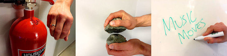
Sound example no. 1

Tapping with a ring on a fire extinguisher.

The sounds are impulsive, with an abrupt start and a slower (but still quite fast) decay. The tapping actions are also impulsive.

Here is a video showing a spectrogram of the sound file. We will look more closely at spectrograms later this week, but for now, notice that for each sound onset, a distinct vertical line is shown in the spectrogram. The horizontal lines that continue from the vertical lines are the partials in the sound.

Sound example no. 2

Rocks rubbed against each other.

Both the actions and sounds are of the sustained type, but if you listen carefully you will notice a grain-like quality to the sound which may be argued to be iterative

The spectrogram of this sound file looks quite different. The vertical lines are less distinct, and do not cover the entire vertical range. This indicates that the sound onset is slower, which is typical for sustained sounds, and that there is less high-frequency content.

Sound example no. 3

Marker pen on white board

Sustained actions and sounds when writing, but with short, impulsive sounds when the pen hits the board

The spectrogram of sound example number 3 is also different. There are impulsive low-frequency sounds each time the marker is put to the whiteboard. The spectrogram shows that the pitched squeeky sounds caused by the marker have more distinct partials than the rest of the sound file.

2.9 Exploring Sound-producing Actions

We shall here look more closely at some terminology used to describe sound-producing actions.

Objects and Actions

Sounds are produced when actions work on two or more objects, what is often called interaction. We may therefore think of this as an object-action-object system, as illustrated in the figure below.

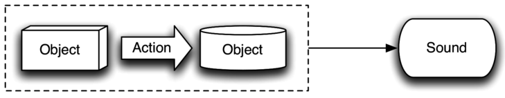
In nature, the features of such a system are defined by the acoustical properties of each of the objects involved in the interaction (such as the size, shape and material), and the mechanical laws of the actions that act upon them (such as the external forces and gravitational pull). It is our life-long experience of acoustical and mechanical properties of objects and actions, that makes us able to predict the sound of an object-action-object system even before it is heard.

Affordance of Sound-producing Actions

To use Gibson’s affordance concept again, we may say that an object-action-object system affords a specific type of sonic result. For example, when we see a drummer hit a drum with her stick, we know that we will hear a drum sound because we have seen (and heard!) drums before. Think of any instrument (or other object for that matter), and you can probably imagine how it will sound.

Even more, you can probably think of many different sound-producing actions to use with one particular instrument, hitting, sliding, blowing, and so on. And you can use many different objects to interact with your instrument, such as a mallet or a bows. As you can easily imagine, there are endless combinations of such action-sound couplings. The remarkable thing is that we are able to imagine and predict the sonic outcome of such couplings. Our main argument here is that this embodied knowledge is deeply rooted in our cognitive system.

From Brain to Sound

So far we have only discussed the perception of sound-producing actions. But we may also think of a chain describing the production of such actions. The figure below shows the action-sound chain from cognitive process to sound, and with feedback in all parts of the chain.

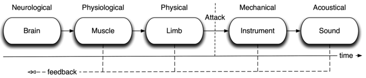
The chain starts with neurological activity in the brain, followed by physiological activity in a series of muscles, and biomechanical activity in limbs of the body. The interaction between the body and the object occurs as an attack when an element of the object (for example a drum membrane) is excited and starts to resonate.

The feedback in the chain is important, as it is part of the action-perception loop. It is this constant feedback from all our parts of the body that make us able to adjust our actions continuously. For example, just think of how a jazz drummer is constinantly able to adapt the playing to make the best sound from the drums and to pick up on the musical elements of the other musicians.

Excitation, Prefix, Suffix

If we zoom in on only the “attack” part of the chain depicted above, it can be seen as consisting of three elements: prefix, excitation and suffix.

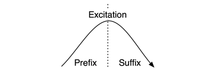
The prefix is the part of a sound-producing action happening before the excitation, and is important for defining the quality of the excitation. The suffix is the return to equilibrium, or the initial state, after the excitation.

The prefix, excitation and suffix are closely related both for the performance and the perception of a sound-producing action. Following the idea of our perception being based on an active action-perception loop, a prefix may guide our attention and set up expectations for the sound that will follow. For example, when we see a percussionist lifting the mallet high above a timpani we will expect a loud sound. We will also expect the rebound of the mallet (the suffix) to match the energy level of the prefix, as well as the sonic result. As such, both prefixes and suffices help to “adjust” our perception of the sound, based on our ecological knowledge of different action-sound types.

Action-Sound Types

The French composer and musicologist Pierre Schaeffer was a pioneer in defining a structured approach to thinking about musical sound. We will here build on his concept of three main types of sounds:

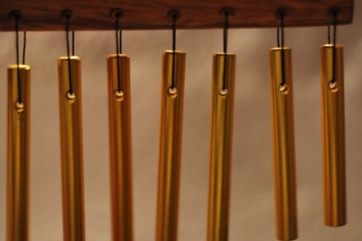
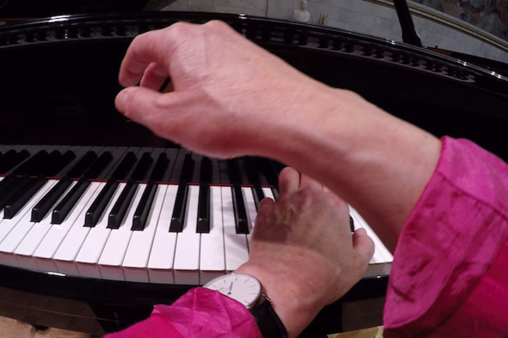
• Impulsive: sounds characterised by a discontinuous energy transfer, resulting in a rapid sonic attack with a decaying resonance. This is typical of percussion, keyboard and plucked instruments.
• Sustained: sounds characterised by a continuous energy transfer, resulting in a continuously changing sound. This is typical of wind and bowed string instruments.
• Iterative: sounds characterised by a series of rapid and discontinuous energy transfers, resulting in sounds with a series of successive attacks that are so rapid that they are not perceived individually. This is typical of some percussion instruments, such as guiro and cabasa, but may also be produced by a series of rapid attacks on other instruments, for example rapid finger actions on a guitar.

It is important to note that many instruments can be played with both impulsive and sustained actions. For example, a violin may be played with a number of different sound-producing actions, ranging from pizzicato to bowed legato. However, the aim of categorising sound-producing actions into three action-sound types is not to classify instruments, but rather to suggest that the mode of the excitation is directly reflected in the corresponding sound.

As shown in the figure below, each of the action-sound types may be identified from the energy profiles of both the action and the sound.

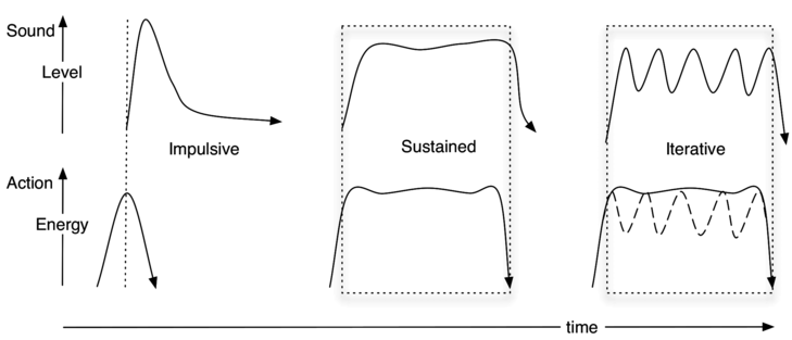
Here the dotted lines indicate where the excitation occurs. Note that two action possibilities are sketched for the iterative action-sound type, since iterative sounds may often be the result of either the construction of the instrument or the action with which the instrument is played. An example of an iterative sound produced by a continuous action can be found in a cabasa, where the construction of the instrument makes the sound iterative. Playing a tremolo, on the other hand, involves a series of iterative actions, but these actions tend to fuse into one superordinate action. In either case, iterative sounds and actions may be seen as having different properties than that of impulsive and sustained action-sound types.

References

• Gibson, J. J. (1979). The Ecological Approach to Visual Perception. Hillsdale, NJ: Lawrence Erlbaum Associates.
• God�y, R. I. (2001). Imagined Action, Excitation, and Resonance. In R. I. God�y & H. J�rgensen (Eds.), Musical Imagery (pp. 237�250). Lisse: Swets and Zeitlinger.
• Jensenius, A. R. (2007). Action�Sound: Developing Methods and Tools to Study Music-Related Body Movement (PhD thesis). University of Oslo.
• Schaeffer, P. (1966). Solf�ge de l�objet sonore. Paris: INA/GRM.

2.11 Introduction to Sound and Movement Analysis

In this week’s methods track we will explore qualitative movement analysis and learn about sound analysis.

As we saw last week, there are many ways of analysing music-related body motion. The qualitative methods are often based on descriptive approaches, and using text as the medium. Several structured approaches to this exist, and in the following video we will look more closely at two systems used for qualitative movement analysis: Labanotation and Laban Movement analysis.

When researching music and movement we need tools for analysing both movement and sound. So after the qualitative movement analysis video you will learn about how it is possible to carry out systematic studies on musical sound. This includes an overview of different visualisation techniques, such as waveform displays and frequency spectra.

2.12 Qualitative movement analysis

In this video you will learn about different types of qualitative movement analysis.

We will in particular look more into two systems developed by dance-choreographer Rudolph Laban: the Labanotation and the Laban Movement Analysis. These systems have not received wide-spread usage, but they are probably the two most well-known notation and analysis methods in use in dance and beyond.

• Video: 2.12 Qualitative movement analysis

2.13 Exploring Sound Analysis

This article introduces some basic techniques for quantitative sound analysis. Most importantly, we will have a look at three visual representations of sound: The waveform, spectrum and spectrogram.

We will only scratch the surface of the vast topic of sound analysis, and you are not required to memorise the technical details given here. However, it is useful to have a conceptual idea of the ways in which sound is analysed and visualised. You may want to first read quickly through this article, then look at the video in the next step, and come back to this article for reference.

Sound waves in the air

What happens if you throw a stone into water? As the stone hits the surface, waves spread from the point of impact. A sound in the air is quite similar. However, the waves are not variations in the water. A sound is variations in air pressure above and below the normal air pressure level. Just like the waves in the water, the sound waves spread out from the source, albeit quite fast; approximately 340 meters (1000 ft) every second. In the image below, the sound wave is displayed with dark areas where the air is more compressed, and light areas where the air is less compressed (the air molecules are more dispersed).

Imagine that you are standing on the blue “x” in the picture above. We can make a graph of the air pressure at your location, such as the example below. Notice that it starts with a steady air pressure (no sound), and then starts to vary once the sound waves hit you.

The variations in air pressure that we perceive as sound are very rapid. We call the speed of these variations the sound frequency. The lowest audible bass frequencies vary 20 times per second (20 Hertz) and the highest audible frequency to a young person without hearing loss is around 20 000 times per second (20 000 Hertz). The amplitude of the sound wave describes how large its pressure variations are. A quick demonstration of frequency and amplitude is shown in this video.

Waveform

The most common way of representing sound is the one you will meet in most types of sound recording software: the waveform. The waveform is actually quite similar to the previous figure. A waveform representation shows how the amplitude (y-axis) of a sound varies over time (x-axis). The figure below shows a waveform representation of a very short sound segment. Time is shown along the horizontal axis. Notice how the amplitude varies above and below the 0 line.

The figure above shows a very short (3 millisecond) excerpt of a sound file. If we “zoom out” of the image, these variations become so small that they “merge” into the blue solid areas in the figure below. We are now unable to see the individual fluctuations from the previous figure, but we can identify several “bursts” of sound.

Frequency content

Natural sounds contain a range of frequencies. Tonal sounds contain a fundamental frequency and a range of overtones which are multiples of the fundamental frequency. For instance a tone with a fundamental frequency of 220 Hertz (called small A), has overtones at 440 Hz, 660 Hz, 880 Hz, etc. Normally, we cannot hear the individual overtones. The fundamental frequency and the overtones fuse together, and their amplitude relationship plays an important role in determining the perceived timbre of the tone. Timbre, sometimes called tone colour, is what makes it possible to distinguish between for instance a flute and a violin who are playing the same tone.

Spectrum

A spectrum representation shows the frequency content of a sound recording. Here the frequency is shown on the horizontal x-axis, and amplitude on the vertical y-axis. The figure below shows a spectrum of a saxophone tone. The peaks in the spectrum are the fundamental frequency and the overtones of the saxophone sound.

Spectrogram

If we are interested in analysing how the spectrum varies over time, we may use what is called a spectrogram (or sometimes sonogram)

A spectrogram is created by dividing the sound file into many short segments, calculating the spectrum for each segment, and placing these next to each other. The picture below shows the conceptual construction of a spectrogram. Essentially, the spectrum of each segment is tilted sideways and colour-coded. The result of placing these colour-columns next to each other is an image showing the variation in frequency content over time.

The picture below shows a spectrogram of the same saxophone melody as shown in the video on sound analysis in the next step.

Sound descriptors

Sometimes we need more precise descriptions of a sound file than we can get from a visual inspection of a waveform or spectrogram. We may then move over to quantitative analysis using sound descriptors. A sound descriptor is a numerical description of a single aspect of the sound. The descriptor may be global, describing an entire sound, or time-varying, describing variations within the sound.

Examples of descriptors

• In a sense, duration is a global descriptor. A sound has a duration which may be described globally with a single number.
• Sound energy as a global descriptor is a description of the total sound energy in the sound file. This is typically found by calculating the root-mean-square value of the waveform. Sound energy may also be a time-varying descriptor. Instead of calculating the energy of the entire sound file, the energy is calculated for a sequence of short time-windows. One number is calculated per time-window, resulting in a sequence of numbers.
• The spectral centroid is often explained as the “centre of gravity” of the spectrum. The time-varying spectral centroid usually reflects how the brightness of the sound evolves over time. The resulting sequence of numbers can be displayed in a plot such as in the picture below.

• Spectral flux describes how much the spectrum varies over time
• Roughness describes a dissonance in the sound that is the result of certain limitations in our auditory system (critical bandwidth)

Software

There exists a wide range of software for sound analysis. Here is a selection of free software that you may try yourself:

• Sonic Visualiser � Free and user-friendly tool for visualising audio files. (Windows / Mac)
• Audacity � Free software for recording and editing multitrack audio. (Windows / Mac)
• Praat � Free software for audio analysis. Mainly targeted at speech analysis but also useful for other types of musical sound. (Windows / Mac)
• Spear � Free software that lets you analyse and manipulate individual sinusoidal components of a sound file. (Mac)
• SpectrumView � Free iOS app producing a simple spectrogram from microphone input. (iOS)

In addition, there exists a range of tools that require a Matlab license. These tools are more advanced, and have a higher threshold to get started:

• MIR Toolbox � Advanced toolbox for audio analysis by Olivier Lartillot. (requires Matlab)
• Timbre Toolbox � Advanced toolbox for audio analysis by researchers from IRCAM and McGill University. (requires Matlab)

2.14 How do we analyse sound?

As for movement analysis, there are both qualitative and quantitative approaches to the analysis of musical sound.

In everyday life, we use words to describe sounds. A sound may be bright, or a song may be sad. Sometimes we need more precise ways to describe sound. In this video you will learn about three different ways of visualising sound: waveform, spectrum, and spectrogram, and also that sounds may be described by means of sound descriptors.

• Video: 2.14 How do we analyse sound?