Chapter 4. Architecture deep dive
Apache Ignite is an open-source memory-centric distributed database, caching and computing platform. It was designed as an in-memory data grid for developing a high-performance software system from the beginning. So its core architecture design is slightly different from that of the traditional NoSQL databases, able to simplify the building of modern applications with a flexible data model and simpler high availability and high scalability.
To understand how to properly design an application with any databases or framework, you must first understand the architecture of the database or framework itself. By getting a better idea of the system, you can solve different problems in your enterprise architecture landscape, can select a comprehensive database or framework that is appropriate for your application and can get maximum benefits from the system. This chapter gives you a look at the Apache Ignite architecture and core components to help you figure out the key reasons behind Ignite’s success over other platforms.
Understanding the cluster topology: shared-nothing architecture
Apache Ignite is a grid technology, and its design implies that the entire system is both inherently available and massively scalable. Grid computing is a technology in which we utilize the resources of many computers (commodity, on-premise, VM, etc.) in a network towards solving a single computing problem in parallel fashion.
Note that there is often some confusion about the difference between grid and cluster. Grid computing is very similar to cluster computing, the big difference being that cluster computing consists of homogeneous resources, while grids are heterogeneous. Computers that are part of a grid can run different operating systems and have different hardware, whereas cluster computers all have the same hardware and OS. A grid can make use of spare computing power on a desktop computer, while the machines in a cluster are dedicated to working as a single unit and nothing else. Throughout this book, we use the terms grid and cluster interchangeably.
Apache Ignite also provides a shared-nothing architecture where multiple identical nodes form a cluster with no single master or coordinator. All nodes in a shared-nothing cluster are identical and run the exact same process. In the Ignite grid, nodes can be added or removed nondisruptively to increase (or decrease) the amount of RAM available. Ignite internode communication allows all nodes to receive updates quickly without having any master coordinator. Nodes communicate using peer-to-peer message passing. The Apache Ignite grid is sufficiently resilient, allowing the nondisruptive automated detection and recovery of a single node or multiple nodes.
On the most fundamental level, all nodes in the Ignite cluster fall into one of two categories: client and server. There is a big difference between the two types of nodes, and they can be deployed in different ways. In the rest of this section, we will talk about the topology of the Ignite grid and how it can be deployed in real life.
Client and server node
An Ignite node is a single Ignite process running in a JVM. Apache Ignite nodes have an optional notion of client and server nodes as we mentioned before. Often, an Ignite client node also addresses as a native client node. Both client and server nodes are part of Ignite’s physical grid and are interconnected with each other. The client and server nodes have the following characteristics.
| Node | Description |
|---|---|
| Server | 1. Acts as a container for storing data and computing. A server node contains data, participates in caching, computing and streaming. 2. Generally starts as a standalone Java process. |
| Client | 1. Acts as an entry point to run operations like put/get into the cache. 2. Can store portions of data in the near cache, which is a smaller local cache that stores most recently and most frequently accessed data. 3. It is also used to deploy compute and service tasks to the server nodes and can participate in computation tasks (optional). 4. Usually embedded with the application code. |
All nodes in the Ignite grid start as server nodes by default, and client nodes need to be explicitly enabled. You can imagine the Ignite client node as a thick client (also called a fat client, e.g., Oracle OCI8). Whenever a client node connects to the Ignite grid or cluster, it is aware of the grid topology (data partitions for each node) and is able to send a request to the particular node to retrieve data. You can configure an Ignite node to be either a client or a server via a Spring or Java configuration, as shown below.
Spring configuration:
<bean class="org.apache.ignite.configuration.IgniteConfiguration">
    ...
    <!-- Enable client mode. -->
    <property name="clientMode" value="true"/>
    ...
</bean>
Java configuration:
IgniteConfiguration cfg1 = new IgniteConfiguration();
cfg1.setGridName("name1");
// Enable client mode.
cfg1.setClientMode(true);
// Start Ignite node in client mode
Ignite ignite1 = Ignition.start(cfg1);
Here is also a special type of logical node called a compute node in the Ignite cluster. A compute node is the node that usually participates in computing business logic. Basically, a server node that contains data is also used to execute computing tasks.
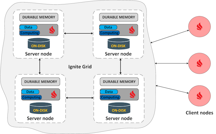
However, an Apache Ignite client node can also participate in computing tasks optionally. The concept might seem complicated at first glance, but let’s try to clarify it.
Server nodes or Data nodes always stores data and participating in any computing task. On the other hand, the Client node can manipulate the server caches, store local data and optionally participate in computing tasks. Usually, client nodes are only used to put or retrieve data from the caches.
Why should you want to run any computing task on client nodes? In some cases (for instance high volume transactions in the server nodes), you do not want to execute any job or computing task on the server nodes. In such a case, you can choose to perform jobs only on client’s nodes by creating a cluster group. This way, you can separate the server node (data node) from the nodes that are particular uses for computing in the same grid.
A cluster group is a logical unit of a few nodes (server or client node) that group together in a cluster to perform some work. Within a cluster group, you can limit job execution, service deployment, streaming and other tasks to run only within a cluster group. You can create a cluster group based on any predicate. For instance, you can create a cluster group from a group of nodes, where all the nodes are responsible for caching data for a cache named testCache. It’s enough for now, and we will explore this distinction later in the subsequent section of this chapter.
Ignite nodes can be divided into two major groups from the deployment point of view:
- Embedded with the application.
- Standalone server node.
Embedded with the application
Apache Ignite as a Java application can be deployed embedded with other applications. It means that Ignite nodes will be runs on the same JVM that uses the application. Ignite node can be embedded with any Java web application artifact like WAR or EAR running on any application server or with any standalone Java application. Our HelloIgnite Java application from chapter 2 is a perfect example of embedded Ignite server. We start our Ignite server as a part of the Spring application running on the same JVM and joins with other nodes of the grids in this example. In this approach, the life cycle of the Ignite node is tightly bound with the life cycle of the entire application itself. Ignite node will also shut down if the application dies or is taken down. This topology is shown in figure 4.3.
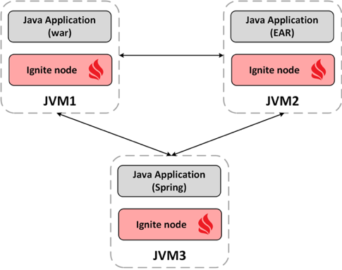
If you change the IgniteConfiguration.setClientMode property to false, and rerun the HelloIgnite application, you should see the following:

HelloIgnite Java application run and joins to the cluster as a server node. The application exists from the Ignite grid after inserting a few datasets. Another excellent example of using Ignite node as an embedded mode are implementing web session clustering. In this approach, you usually configure (web.xml file) your web application to start an Ignite node in embedded mode. When multiple application server instances are running, all embedded Ignite nodes connect with each other and forming an Ignite grid. Please see the chapter 5 Intelligent caching for more details of using web session clustering.
Client and the server nodes in the same host
This is one of the typical cases when Ignite client and server nodes are running on different JVM in the same host. You can execute Ignite client and server nodes in separate containers such as Docker or OpenVZ if you are using container technology for running JVM. Both containers can be located in the same single host.
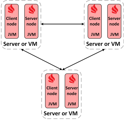
The container isolates the resources (CPU, RAM, Network interface) and the JVM only uses isolated resources assigned to this container. Moreover, the Ignite client and server node can be deployed in the separate JVM in the single host without containers, where they all use the shared resourced assigned to this host machine. Host machine could be any on-premise, virtual machine or Kubernates pods.
Running multiple nodes within single JVM
It is possible to start multiple nodes from within a single JVM. This approach is very popular for unit testing among developers. Ignite nodes running on the same JVM connects with each other and forming an Ignite grid.
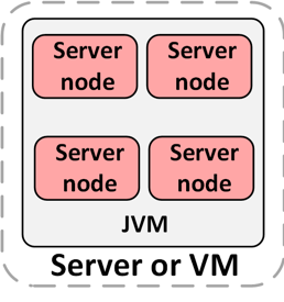
One of the easiest ways to run a few nodes within a single JVM is by executing the following code::
IgniteConfiguration cfg1 = new IgniteConfiguration();
cfg1.setGridName("g1");
Ignite ignite1 = Ignition.start(cfg1);
IgniteConfiguration cfg2 = new IgniteConfiguration();
cfg2.setGridName("g2");
Ignite ignite2 = Ignition.start(cfg2);
Real cluster topology
In this approach Ignite client and server nodes are running on different hosts. These are the most common way to deploy a large-scale Ignite cluster for production use because it provides greater flexibilities in term of cluster technics. Individual Ignite server node can be taken down or restarted without any impact to the overall cluster.
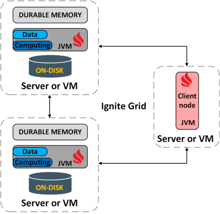
Such a cluster can be quickly deployed in and maintained by the kubernates which an open source system for automating deployment, scaling, and management of the containerized application. VMWare is another common cluster management system rapidly used for the Ignite cluster.
Data partitioning in Ignite
Data partitioning is one of the fundamental parts of any distributed database despite its storage mechanism. Data partitioning and distribution technics are capable of handling large amounts of data across multiple data centers. Also, these technics allow a database system to become highly available because data has been spread across the cluster.
Traditionally, it has been difficult to make a database highly available and scalable, especially the relational database systems that have dominated the last couple of decades. These systems are most often designed to run on a single large machine, making it challenging to scale out to multiple machines.
At the very high level, there are two styles of data distribution models available:
- Sharding: it’s sometimes called horizontal partitioning. Sharding distributes different data across multiple servers, so each server act as a single source for a subset of data. Shards are called partitions in Ignite.
- Replication: replication copies data across multiple servers, so each portion of data can be found in multiple places. Replicating each partition can reduce the chance of a single partition failure and improves the availability of the data.
Usually, there are several algorithms uses for distributing data across the cluster, a hashing algorithm is one of them. We will cover the Ignite data distribution strategy in this section, which will build a deeper understanding of how Ignite manages data across the cluster.
Understanding data distribution: DHT
As you read in the previous section, Ignite shards are called partitions. Partitions are memory segments that can contain a large volume of a dataset, depends on the capacity of the RAM of your system. Partition helps you to spread the load over more nodes, which reduces contention and improves performance. You can scale out the Ignite cluster by adding more partitions that run on different server nodes. The next figure shows an overview of the horizontal partitioning or sharding.
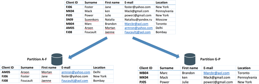
In the above example, the client profile’s data are divided into partitions based on the client Id key. Each partition holds the data for a specified range of partition key, in our case, it’s the range of the client ID key. Note that, partitions are shown here for the descriptive purpose. Usually, the partitions are not distributed in any order but are distributed randomly.
Distributed Hash Table or DHT is one of the fundamental algorithms used in the distributed scalable system for partitioning data across the cluster. DHT is often used in web caching, P2P system, and distributed database. The first step to understand the DHT is Hash Tables. Hashtable needs key, value, and one hash function, where hash function maps the key to a location (slot) where the value is located. According to this schema, we apply a hash function to some key attribute of the entity we are storing that becomes the partition number. For instance, if we have four Ignite nodes and 100 clients (assume that client Id is a numeric value), then we can apply the hash function hash (Client Id) % 4, which will return the node number where we can store or retrieve the data. Let’s begin with some basic details of the Hashtable.
The idea behind the Hashtable is straightforward. For each element we insert, we have to have calculated the slot (technically, each position of the hash table is called slot) number of the element into the array, where we would like to put it. Once we need to retrieve the element from the array, we recalculate its slot again and returns it’s as a single operation (something like return array [calculated index or slot]). That’s why it has O(1) time complexity. In short, O(1) means that the operation takes a certain (constant) amount of times, like 10 nanoseconds or 2 milliseconds. The process of calculating unique slot of each element is called Hashing and the algorithm how it’s done called Hash function.
In a typical Hash table design, the Hash function result is divided by the number of array slots and the remainder of the division becomes the slot number of the array. So, the index or slot into the array can be calculated by hash(o) % n, where o is the object or key, and n is the total number of slots into the array. Consider the following illustration below as an example of the hash table.
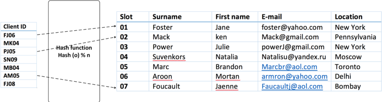
The value on the left represents keys in the preceding diagram, which are being hashed by the hash function for producing the slot where the value is stored. Based on the hash value computed, all the items placed in respective slots. Also, we can look up the client profile of a given client Id by calculating its hash and then accessing the resulting slot into the array.
Hash table is well suited for storing data set allocated in one machine. However, when you have to accommodate a large number of keys, for instance, millions and millions of keys, DHT comes into play. A DHT is merely a key-value store distributed across many nodes in a cluster. You have to divide the keys into subsets of keys and map those keys to a bucket. Each bucket will reside in a sperate node. You can assume a bucket as a sperate hash table. In one word, using buckets to distribute the key-value pairs is DHT.
Another key objective of the hash function in a DHT is to map a key to the node that owns it, such that a request can be made to the correct node. Therefore, there are two hash functions for looking up the value of the key across the cluster in DHT. The first hash function will search for the appropriate bucket maps to the key, and the second hash function will return the slot number of the value for the key located in the node. We can visualize the schema as shown in figure 4.9.
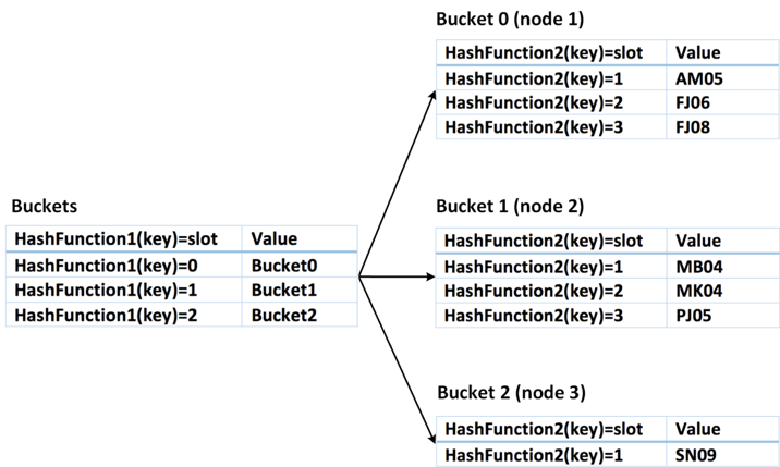
To illustrate this, we modified our previous hash table to store pointers to the bucket instead of values. If we have three buckets as shown in the preceding example, then key=1 should go to the bucket 1, key=2 will go to bucket 2 and so on. Therefore, we have to need one more hash function to find out the actual value of the key-value pair inside a particular bucket. HashFucntion2 is the second hash function for looking up the actual key-value pair from the bucket in this case.
Table named Buckets on the left-hand side in figure 4.9 sometimes called partition table. This tables stores the partition IDs and the node associated to that partition. The function of this table is to make all members of the entire cluster aware of this information, making sure that all members know where the data is.
The fundamental problem of DHT is that it effectively fixes the total number of the nodes in the cluster. Adding a new node or removing nodes from the cluster means changing the hash function which would require redistribution of the data and downtime of the cluster. Let’s see what happens when we remove the bucket 2 (node 3) from the cluster, the number of buckets is now equal to two, i.e., n=2. This changes the result of the hash function hash (key) % n, causing the previous mapping to the node (bucket) unstable. The key=2 which was previously mapped to bucket two now mapped to bucket 0 since key % 2 is equal to 0. We need to move the data between buckets to make it still work, which is going to be expensive in this hashing algorithm.
A workaround for this problem is to use Consistence Hashing or Rendezvous hashing. Often Rendezvous hashing is also called Highest Random Weight (HRW) hashing. Apache Ignite uses the Rendezvous hashing, which guarantees that only the minimum amount of partitions will be moved to scale out the cluster when topology changes.
Rendezvous hashing
Rendezvous hashing (aka highest random weight (HRW) hashing) was introduced by David Thaler and Chinya Ravishankar in 1996 at the University of Michigan. It was first used for enabling multicast clients on the internet to identify rendezvous points in a distributed fashion. It was used by Microsoft corporation for distributed cache coordination and routing a few years later. Rendezvous hashing is an alternative to the ring based, consistent hashing. It allows clients to achieve distributed agreement on which node a given key is to be placed in.
The algorithm is based on a similar idea of consistent hashing where nodes are converted into numbers with hash. The basic idea behind the algorithm is that the algorithm uses weights instead of projecting nodes and their replicas on a circle. A numeric value is created with a standard hash function hash(Ni, K) to find out which node should store a given key, for each combination of the node (N) and key (K). The node that’s picked is the one with the highest number. This algorithm is particularly useful in a system with some replication (we will detail the replication mechanism in the next section, for now, data replication is a term means to have redundancies data for high availability) since it can be used to agree on multiple options.
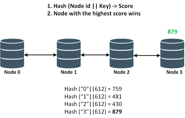
Both Consistent hashing and Rendezvous hashing algorithms can be used in a distributed database to decide the home node for any given key, and often can replace each other. However, Rendezvous hashing or HRW have some advantages over Consistent hashing (CH).
- You do not have to pre-define any tokens for the nodes to create any circle for HRW hashing.
- The biggest advantage of the HRW hashing is that it provides a very even distribution of keys across the cluster, even while nodes are being added or removed. For CH, you have to create a lot of virtual nodes (Vnodes) into each node to provide evenly distribution of keys on a small size of a cluster.
- HRW hashing doesn’t store any additional information for data distribution.
- Usually, HRW hashing can provide different N servers for a given key K. This makes it very useful to support storing redundant data.
- Finally, HRW hashing is simple to understand and code.
HRW hashing also has a few disadvantages as follows:
- HRW hashing requires more than one hashing computation per key to maps key to a node. It can make a massive difference if you are using some sort of slow hashing function.
- HRW hashing can be slower to run hash functions against each key node combinations instead of the just once with the CH algorithms.
Rendezvous Hashing or HRW hashing is the default algorithm in Apache Ignite for a key to node mapping since version 2.0. RendezvousAffinityFunction class is the standard implementation of the Rendezvous Hashing in the Apache Ignite. This class provides affinity information for detecting which node (nodes) are responsible for the particular key in the Ignite grid.
Mapping of a given key in Ignite is a three steps operation. First, any given key will get an affinity key by using CacheAffinityKeyMapper function. Affinity key will be used to determine a node on which this key will be cached. The second step will map the affinity key to partition using AffinityFunction.partition(object) method. Here, a partition is simply a number from a limited set (0 to 1024), 1024 is default. A key to partition mapping does not change over the time. The third step will map an obtained partition to nodes for the current grid topology version. Partition to node mapping is calculated by using assignPartitions() method, which assigns a collection of nodes to each partition.
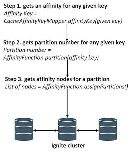
Apache Ignite affinity function (key to node mapping) is fully pluggable, and you can implement your version of Rendezvous Hashing or consistent hashing to determine an ideal mapping for the partition to nodes in the grids. You must have implemented the Java interface AffinityFuction and configure this function in the cache configuration as shown below:

Durable memory architecture
The Ignite new memory architecture as well as native persistence was debuted on version 2.0 and distributed from the end of the last year. The data in memory and on disk has the same binary representation. This means that no additional conversion of the data is needed while moving from in memory to disk. Ignite new memory architecture provides off-heap data storage in a page format. Sometimes it’s also called page-based memory architecture that is split into pages of fixed size. The pages are allocated in managed off-heap (outside of the Java heap) region of the RAM and organized in a particular hierarchy. Let’s start with the basic of the durable memory architecture: page, the smallest unit of the data with a fixed size.
Page
A page is a basic storage unit of data that contains actual data or meta-data. Each page contains a fixed length and has a unique identifier: FullPageId. As mentioned earlier, Pages are stored outside the Java heap and organized in RAM. Pages interact with the memory using the PageMemory abstraction. It usually helps to read, write a page and even allocate a page ID.
When the allocated memory exhausted and the data are pushed to the persistence store, it happens page by page. So, a page size is crucial for performance, it should not be too large, otherwise, the efficiency of swapping will suffer seriously. When page size is small, there could be another problem of storing massive records that do not fit on a single page. Because, to satisfy a read, Ignite have to do a lot of expensive calls to the operating system for getting small pages with 10-15 records.
When the record does not fit in a single page, it spreads across several pages, each of them stores only some fragments of the record. The downside of this approach is that Ignite has to look up the multiple pages to obtain the entire records. So, you can configure the size of the memory page in such cases.
Size of the page can be configured via DataStorageConfiguration.setPageSize(..) parameter. It is highly recommended to use the same page size or not less than of your storage device (SSD, Flash, etc.) and the cache page size of your operating system. Try a 4 KB as page size if it’s difficult to figure out the size of the cache page size of your operating system,.
Every page contains at least two sections: header and page data. Page header includes the following information’s:
- Type: size 2 bytes, defines the class of the page implementation (ex. DataPageIO, BplusIO)
- Version: size 2 bytes, defines the version of the page
- CRC: size 4 bytes, defines the checksum
- PageId: unique page identifier
- Reserved: size 3*8 bytes
Ignite memory page structure illustrated in the following figure 4.29.

Memory pages are divided into several types, and the most important of them are Data Pages and Index Pages. All of them are inherited from the PageIO. We are going to details the Data Page and the Index Page in the next two subsections.
Data Page
The data pages store the data you enter into the Ignite caches. If a single record does not fit into a single data page, it will be stored into several data pages. Generally, a single data page holds multiple key-values entries to utilize the memory as efficiently as possible for avoiding memory fragmentation. Ignite looks for an optimal data page that can fit the entire key-value pair when a new key-value entry is being added to the cache. It makes sense to increase the page size if you have many large entries in your application. One thing we have to remember is that data is swapped to disk page by page and the page is either completely located in RAM or into Disk.

During an entry updates, if the entry size exceeds the free space available in the data page, then Ignite will look for a new data page that has enough space to store the entry and the new value will be moved there. Data page has its header information in addition to the abstract page. Data page consist of two major sections: the data page header and data page data. Data page header contains the following information’s and the structure of the data page is illustrated in figure 4.29.
- Free space, refers to the max row size, which is guaranteed to fit into this data page.
- Direct count.
- Indirect count.
The next portions of data after the page header is data page data and consists of items and values. Items are linked to the key-value. A link allows reading key-value pair as an Nth item in a page. Items are stores from the beginning to the end, and values are stores on reverse order: from the end to beginning.
Index pages and B+ trees
Index pages are stored in a structure known as a B+ tree, each of them can be distributed across multiple pages. All SQL and cache indexes are stored and maintained in B+ tree data structure. For every unique index declared in SQL schema, Ignite initialized and managed a dedicated B+ tree instance. Unlike data pages, index pages are always stored in memory for quick access when looking for data.
A B+ tree structure is very similar to a B tree with the difference that an additional level is added at the bottom with linked leaves. The purpose of the B+ tree is to link and order the index pages that are allocated and stored within the durable memory. This means that only a small number of pointers or links traversal is necessary to search for value if the number of the keys in a node is very large. Finally, the index pages of the B+ tree all contain a next sibling pointer for fast iteration through a contiguous block of value. This allows for extremely fast range queries.
In B+ tree binary search is used to find out the required key. To search for an element into the tree, one load up the root nodes finds the adjacent keys that the searched-for value is between. If the required value is not found, it is compared with other values in the tree.
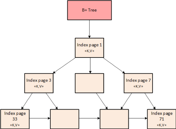
There is a high cost of allocating memory for a large number of pages including data or index pages, which solves through the next level of abstraction called Segments.
Segments
Segments are a contiguous block of physical memory, which are the atomic units of the allocated memory. When the allocated memory runs out, the operating system is requested for an additional segment. Further, this segment is divided into pages of fixed size. All page types include data or index pages resides in the segment.

It is possible to allocate up to 16 memory segments for one dedicated memory region with the size of the segments at least 256 MB in the current version. Ignite uses a particular component for managing information about pages currently available in memory segment and page Id mapping to region address called LoadedPagesTable. LoadedPagesTable or PageIdTable manages mapping from Page ID to relative memory segment chunk (unsafe). LoadedPagesTable uses Robin Hood Hashing algorithm for maintaining HashMap of FullPageId since Ignite version 2.5.
When it comes about memory segment, it is necessary to mention the memory consumption limits. In Apache Ignite data are stored in caches. Obviously, we cannot keep the entire dataset forever in memory. Also, different data may have different storage requirements. To make it possible to set limits at the level of each cache, a hybrid approach was chosen that allows Ignite to define limits for groups of caches, which brings us to the next level of abstraction called memory Region.
Region
The top level of the Ignite durable memory storage architecture is the data Region, a logical expandable area. Data region can have a few memory segments and can group segments that share a single storage area with their settings, constraints and so on. Durable memory architecture can consist of multiple data regions that can vary in size, evictions policies and can be persisted on disk.
Data region encapsulates all the data storage configuration for operational and historical data for your utilization in Ignite and can have one or more caches or tables on a single region. With data region configuration you can manage more than one data region, which can be used for storing historical and operation data of your system. There are different cases when you might do this. The most trivial example is that when you have different non-related caches or tables with different limits.
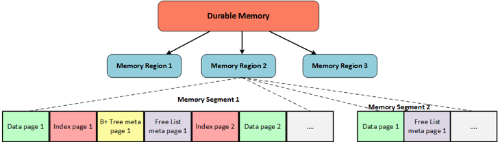
Let’s assume that in our application we have Product, Purchase history entities stored in ProductCache and PurchaseHistCache caches respectively. Here, the Product data is operational and access by the application frequently. Moreover, the Purchase History data needed occasionally and not very critical to lose. In this situation, we can define two different regions of memory with different sizes: Data_region_4GB and Data_region_128GB.
- Data_region_128GB is only 128 GB of memory and will store the operational or frequently access data such as Products.
- Data_region_4GB size is 4 GB and will be allocated for rarely accessed data sets like Purchase history.
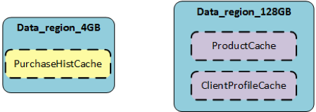
When we create caches, we should have specified the region, on which the cache will belong to. The limits here are applied on the data region level. When you put or insert something in your small cache, and if you exceed the maximum size of the data region (ex. 4 GB), you will get out of the memory (IgniteOutOfMemory) exception, even when the larger data region is empty. You can’t use the memory that is allocated for the Data_region_128GB by the small caches, because it is assigned to the different data region.
So, you should remove or swap the stale data from the data region if you want to avoid this out of memory error. For these circumstances, Ignite provides a few data eviction algorithms to remove unnecessary data from in memory.
Ignite read/write path
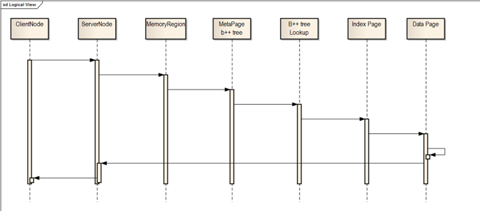
Ignite uses a B+ tree index to find out the potential data pages to fulfil a read. Ignite processes read data at several stages on the read path to discover where the data is stored, starting looking up the key in the B+ tree and finishing with data page:
- On the client node, a cache method has been called
myCache.get(keyA). - Client node identifies the server node that is responsible for this given key
keyAusing the built-in affinity function and delegates the request to the server node over the network. - The server node determines the memory region that is responsible for the cache
myCache. - In the corresponding memory region, a request goes to the meta page, which contains the entry points to a B+ tree by the key of this cache.
- Based on the
keyAhash code, the index page the key belongs to will be located in the B+ tree. - Ignite will return a null value if the corresponding index page is not found in the memory or on the disk.
- If the index page exists, then it contains the reference to the data page of the entry
keyA. - Ignite accesses the data page for keyA and returns the value to the client node.
The above schema for data looks up by the key can be illustrated as shown in figure 4.38.
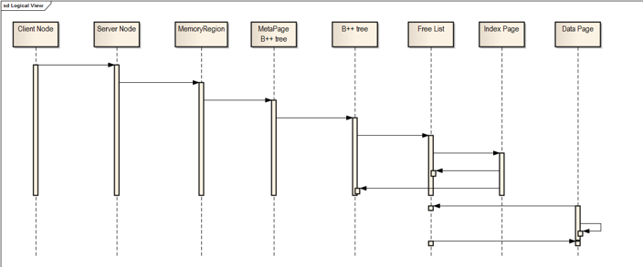
Similar to the read path, Ignite processes data at several stages on a write path. The only difference is that, when a write occurs, Ignite looks for the corresponding index page in the B+ tree. If the index page is not found, Ignite requests a new index page from one of the free lists. The same thing happens for the data page. Also, a new data page also requests from the free list.
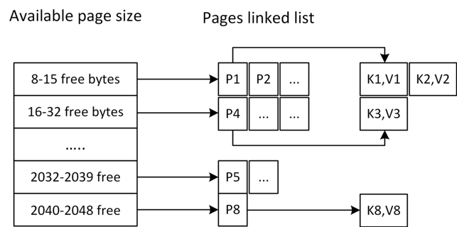
Free List is a list of pages, structured by an amount of space remained within a page. Ignite manages free lists to solve the problem of fragmentation in pages (not full page). Free lists make the allocation and deallocation operations of the data and index pages straightforward, and allow to keep track of free memory. For instance, the image in figure 4.39 shows a free list that stores all the data pages that have up to 15% free space available. Data and index pages are tracked in separate free lists. The list is traversed, and the data/index page that is large enough to store the data is returned when a request for a data/index pages is sent.
Let’s see what’s going under the hood when a myCache.put(keyA, valueA) request sent to the Ignite node:
- A cache method
myCache.put(keyA, valueA)has been called on the client node. - Client node identifies the server node that is responsible for this given key
keyAusing the built-in affinity function and delegates the request to the server node over the network. - The server node determines the memory region that is responsible for the cache
myCache. - A request goes to the Meta page in the corresponding memory region, which contains the entry points to a B+ tree by the key of this cache.
- Based on the
keyAhash code, the index page the key belongs to will be located in the B+ tree. - If the corresponding index page is not found in the memory or on disk, then a new page will be requested from one of the free lists. Once the index page is provided, it will be added to the B+ tree.
- If the index page is empty (i.e., does not refer to any data page), then the data page will be provided by one of the free lists, depending on the total cache entry size. During the selection of the data page for storing the new key-value pair, Ignite does the following:
- Consult marshaller about size in bytes of this value pair.
- Upper-round this value to be divisible by 8 bytes.
- Use the value from the previous step to get page list from the free list.
- Select some page from an appropriate list of free pages. This page will have required amount of free space.
- A reference to the data page will be added to the index page.
- The cache entry is added to the data page.
The Ignite write path with several stages illustrated in the following sequence diagram.
Write-Ahead-Log (WAL)
The Write-Ahead-Log or WAL is a commonly used technique in the database system for maintaining atomicity and durability of writes. The key behind the WAL is that before making any changes to database state, first, we have to log the complete set of operations to the nonvolatile storage (e.g., disk). By writing the log into WAL first, we can guarantee the data durability. If the database crash during changes to the disk, we will be able to read and replay the instructions from the WAL to recover the mutation.
From the Apache Ignite perspective, WAL is a dedicated partition file stored on each cluster node. The update is not directly written to the appropriate partition file but is appended to the end of the WAL file when data are updated in RAM. WAL provides superior performance when compared to in-place updates.
So, what exactly is a Write-Ahead-Log (WAL) file and how it works? Let’s consider an application that’s trying to change the value of A and B from the following four key-values:
(K, V) = (A, 10);
(K, V) = (B, 10);
(K, V) = (C, 20);
(K, V) = (D, 30);
The application is performing an addition of 10 within a single transaction as shown below.
A := A+ 10;
B := B + 10;
The problem arises when there is a system failure during writing to the disk. Assume that, after output(A) on disk, there is a power outage, so output(B) does not get executed, and the value of B is now in the inconsistent state. Value of A on disk is 20, and the value of B is still 10. Therefore, the database system needs a mechanism to handle such failures since they cannot be prevented from any power outage or system crash.
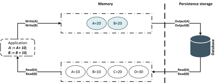
Most database system uses a log-based database recovery mechanism to solve the above problem. A log is the most commonly used structure for recording database modification. The DBMS has enough information available to recreate the original data changes after a crash after the log file has been flushed to disk.
The first log approach is the UNDO log. The purpose of the undo log is to reverse or undo the changes of an incomplete transaction. In our example, during recovery, we have to put the database in the state it was before this transaction, means that changes to A are undone, so A is once again 10 and A=B=10. The undo log file always written to the nonvolatile storage.
Undo logging rules:
- Record a log in undo log file for every transaction T. Write (start T).
- For every action, generate an undo log record with the old value. Write (T, X, VOLD).
- Flush the log to disk.
- Write all the database changes to disk if transaction T commits.
- Then write (commit T) to the log on disk as soon as possible.
An undo log looks very similar as shown in the figure 4.43.
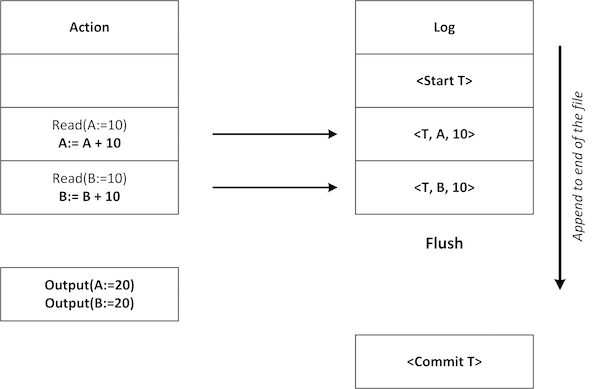
We log a record indicates that we have started the transaction before starting the transaction. When we update the value A, we also write a log indicates its old value 10. Similarly, we record its old value of 10 when we change the value of B from 10 to 20. We flush the undo log to disk before outputting values of A and B to disk. Then we output(A) and output(B) to disk, only after that, we can record (commit T) into undo log file.
Undo logging recovery rules:
- We only undo the failed transaction. If there’s already (commit T) or (abort T) record, do nothing.
- For all (T, X, VOLD):
- output(VOLD)
- write (abort T) to undo log.
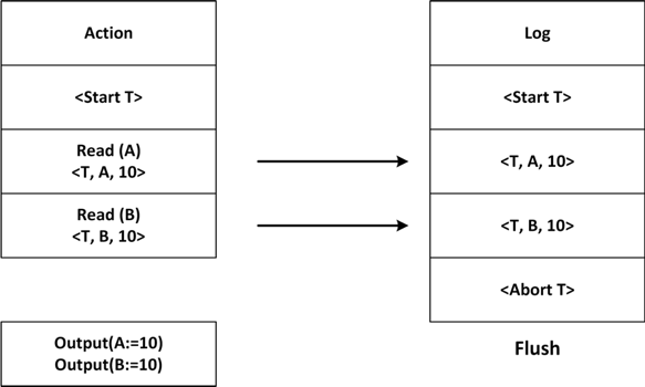
We read the undo log from the end to start, and looking for an incomplete transaction during the recovery process. Any records with (commit T) or (abort T) are ignored because we know that (commit T) or (abort T) can only be recorded after a successful output to disk. We cannot be sure that output was successful if there are no (commit T) record, so for every record, we use the old value VOLD to revert the changes. So, (T, B, 10) sets B back to 10 and so on. Undo log records (abort T) to indicate that we aborted the transaction after making the changes.
The main disadvantage of the undo log is that it might be slower for heavy write-intensive application because for every transaction, we have to output the value to the disk before records a (commit T) log in the undo log file.
At this moment, we can get back to our starting point about WAL. The second log approach for protecting data-loss is the write-ahead log or WAL. Instead of undoing a change, WAL tries to reproduce a change. During the transaction, we write all the changes to WAL that we are indented to do, so we can rerun transaction in case of disaster and reapplying the changes if necessary. Before making any output (write to the disk), we must record the (commit T) record.
WAL logging rules:
- Record a log into undo file for every transaction T. Write (start T) to the log.
- Set its value to New if transaction modifies database record X. Write (T, X, Vnew) to the log.
- Write (Commit T) to the log if transaction T commits.
- Flush the log file to the disk.
- And then, write the new value Vnew for X to disk.
A WAL log file looks something like shown in figure 4.45.
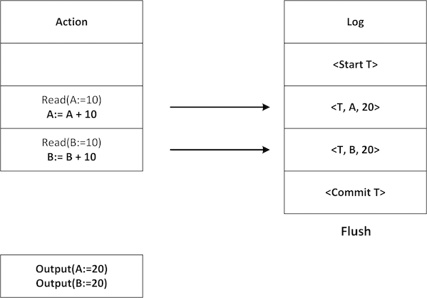
We record the new values for A and B then commit and flush the log to disk. Only after that, we output the values of A and B to the disk. This solves two main issues with disk I/O: buffering and randomly output to disk.
WAL logging recovery rules:
- Do nothing if there’s any incomplete transaction (no commit T) record.
- If there is (commit T), for all (T, X, Vnew):
- output(Vnew)
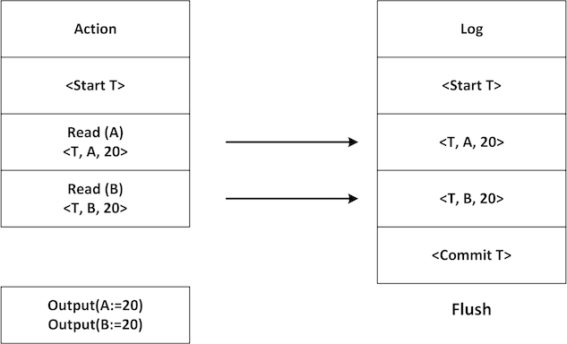
To recover with a WAL log file, we start from the beginning of the file scanning forwards (opposite of the undo log file). If we find any incomplete transaction (no commit T), we skip the transaction so that no output was done. We do not know whether the output was successful or not whenever we find any (commit T) record. In this case, we redo the changes, and even it is redundant. In our example, the value of A will be set to 20, and the value of B will also be set to 20.
Now that we have got the basics of the log structure, so let’s move on to Ignite’s WAL concept to see how the things organized under the cover. From the Ignite perspective, whenever the storage engine wants to make any changes to the data page, it writes the change to the RAM and then appends the changes to the WAL. Storage engine sends an acknowledgment to confirm the operation only after durably written the changes to WAL file on disk.
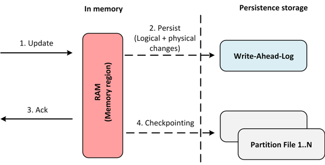
This makes the database changes reliably. If the node crashes while data was being appended to the WAL, no problem because dirty data pages have not been copied from RAM to disk. So, storage engine can read and reply WAL using already saved page set if it crashes while the data pages are being modified. The storage engine can restore to state, which was last committed state of the crashed process. In Ignite, restore is based on page store and WAL log. You may notice that Ignite native persistence is slightly different than the classical WAL log concept.
Baseline topology
Ignite Baseline Topology or BLT represents a set of server nodes in the cluster that persists data on disk.

Where,
- N1-2 and N5 server nodes are the member of the Ignite cluster with native persistence enable that persists data on disk.
- N3-4, N6 server nodes are the member of the Ignite cluster but not a part of the baseline topology.
The nodes from the baseline topology are a regular server node, that store’s data in memory and on the disk, and also participate in computing tasks. Ignite cluster can have different nodes that are not a part of the baseline topology such as:
- Server nodes that are not used Ignite native persistence to persist data on disk. Usually, they store data in memory or persists data to a 3rd party database or NoSQL. In the above equitation, node N3 or N4 might be one of them.
- Client nodes that are not stored shared data.
Let’s start at the beginning and try to understand its goal and which problem it’s solved to clear the baseline topology concept.
The database like Ignite is designed to support massive data storage and processing. Ignite database are highly scalable and fault-tolerant. This high scalability feature of the Ignite brings a few challenges for the database administrator, such as:
- how to manage a cluster?
- How to add/remove nodes correctly? or
- how to rebalance data after add/remove nodes?
Ignite cluster with a multitude of nodes can significantly increase the complexity of the data infrastructure. Let’s look at it by the example of Apache Ignite. Ignite in-memory mode cluster concept is very simple. There are no master or dedicated node in the cluster, and every node is equal. Each node stores a subset of data and can be participated in distributed computing or deploy any services. In case of any node failures, client requests served by the other nodes, and the data of the failed nodes will be no longer available. In this mode, Ignite cluster management operations are very similar as follows:
- To run a cluster, start all nodes.
- To expand the cluster topology, add some nodes.
- To reduce the cluster topology, remove some nodes.
Data redistributes between nodes automatically. Data partitions moves from one node to another depending on the backup copy configuration of the caches.
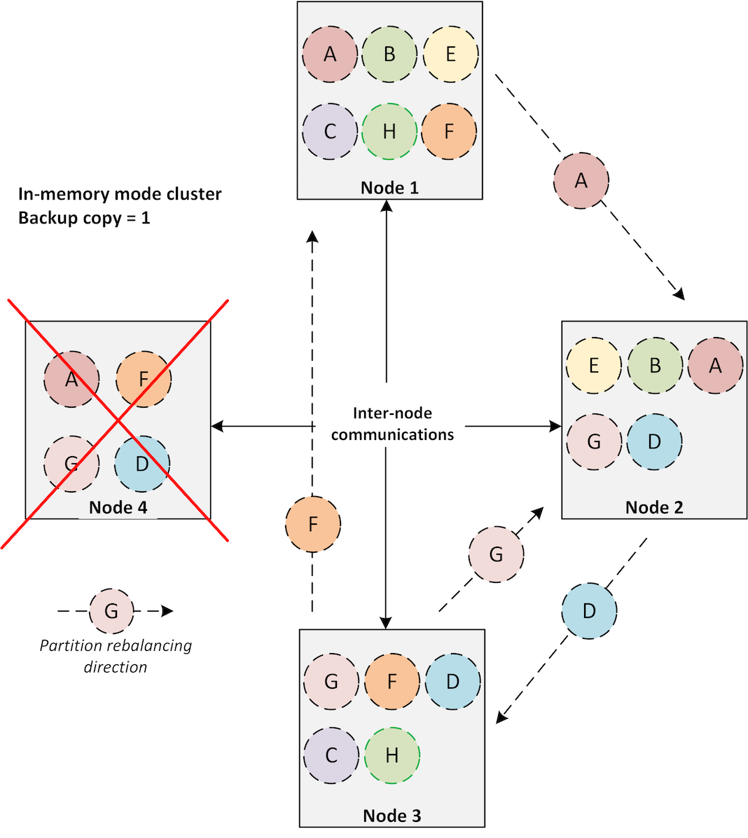
In the persistence mode, the node keeps their state even after the restart. Data is read from the disk and restores the node state during any read operation. Therefore, restart of a node in persistence mode does not need to redistributed data from one node to another unlike in-memory mode. The data during node failure will be restored from the disk. This strategy opens up the opportunities to not only preventing of moving a massive amount of data during node failure but also reduce the startup times of the entire cluster after a restart. So, we need to distinguish somehow these nodes that can save their state after restart. In other words, the Ignite baseline topology provides this capability.
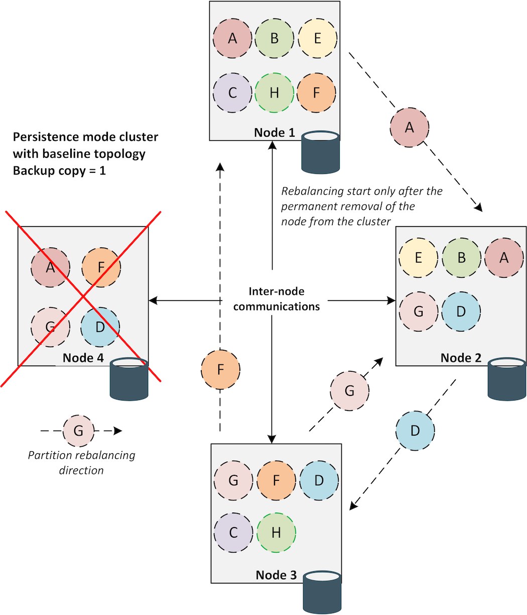
In a nutshell, Ignite baseline topology is a collection of nodes that have been configured for storing persistence data on disk. Baseline topology tracks the history of the topology changes and prevents data discrepancies in the cluster during recovery. Let’s resume the goals of the baseline topology:
- Avoid redundant data rebalancing if a node is being rebooted.
- Automatically activate a cluster once all the nodes of the baseline topology have joined after a cluster restart.
- Prevent the data inconsistencies in the case of split-brain.
Please note that, you can use persistence caches with the in-memory caches at the same time. In-memory caches will live same as before: consider all nodes are equals and begin redistribution of the partitions whenever a node goes down. Baseline topology will take action only on the persistence caches. Hence, Ignite baseline topology has the following characteristics:
- Baseline topology defines a list of nodes which intended for storing data, and does not affect other functionalities such as data grid, compute grid etc. If a new node joined to the cluster where baseline topology is already defined, the data partitions is not started moving to the new node until the node is added to the baseline topology manually.
- On each node, persistence Meta-data repository is used to store the history of the baseline topology.
- For a newly created cluster (or cluster without baseline topology), a baseline topology is created for the first time during the first activation of the cluster. The administrator must explicitly do all the future changes (add/remove nodes) of the baseline topology.
- If baseline topology is defined for a cluster, after restarting the cluster, the cluster will be activated automatically whenever all the nodes from the baseline topology are connected.
Now, let’s details how Ignite storage engine achieves the abovementioned goals.
Automatic cluster activation
A cluster can make on its own decision to activate the cluster in the persistence mode with baseline topology. After the first activation of the cluster, the first baseline topology is created and saved on the disk, which contains information about all nodes present in the cluster at the time of activation. Each node checks the status of the other nodes within the baseline topology after the cluster is rebooted. The cluster is activated automatically once all the nodes are online. This time the database administrator needs no manual intervention to activate the cluster.
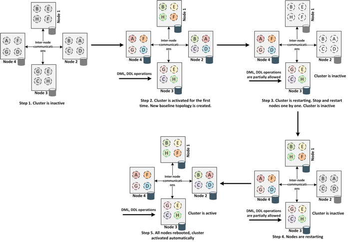
Let’s go through the details of the automatic cluster activation when Ignite persistence is enabled:
- Step 1. All nodes started. The cluster is inactive state and can’t handle any DDL/DML operations (SQL, Key-value API).
- Step 2. The cluster is activated by the database administrator manually. First baseline topology is created, added all the currently running server nodes to the baseline topology.
- Step 3. Database administrator decided to restart the entire cluster to perform any software or hardware upgrade. Administrator stopped or restarted each node one by one.
- Step 4. Nodes are started back one by one and joined to the cluster.
- Step 5. Once all the nodes are baseline topology booted, the cluster gets activated automatically.
Although, Apache Ignite is a horizontally scalable database and nodes can be added and removed from the cluster dynamically, baseline topology proceeds from the concept that in persistence mode the user maintains a stable cluster in production.
Split-brain protection
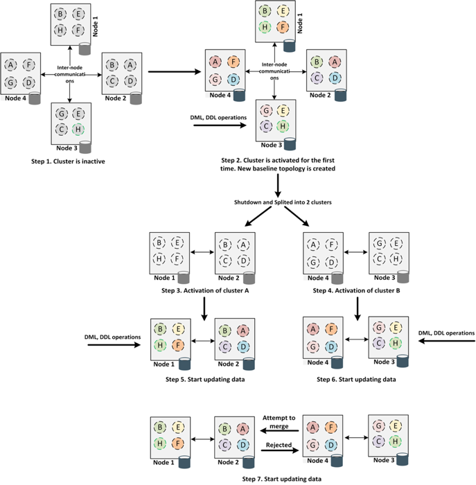
Split-brain is one of the common problems of distributed systems, in which a cluster of nodes gets divided into smaller clusters of equal or nonequal numbers of nodes, each of which believes it is only the active cluster. Commonly, the split-brain situation is created during network interruption or cluster reformation. The cluster reforms itself with the available nodes when one or more node fails in a cluster. Sometimes instead of forming a single cluster, multiple mini clusters with an equal or nonequal of nodes may be formed during this reformation. Moreover, these mini cluster starts handling request from the application, which makes the data inconsistency or corrupted. How it may happen is illustrated in figure 4.56. Here’s how it works in more details.
- Step 1. All nodes started. The cluster is inactive state and can’t handle any DDL/DML operations (SQL, Key-value API).
- Step 2. The cluster is activated by the database administrator manually. First baseline topology is created, added all the currently running server nodes to the baseline topology.
- Step 3. Now let’s say, a network interruption has occurred. Database administrator manually split the entire cluster into two different clusters: cluster A and cluster B. Activated the cluster A with a new baseline topology.
- Step 4. Database administrator activated the cluster B with a new baseline topology.
- Step 5-6. Cluster A and B are started getting updates from the application.
- Step 7. After a while, the administrator resolved the network problem and decided to merge the two different cluster into a single cluster. In this time baseline topology of the cluster A will reject the merge, and an exception will occur as follows:
class org.apache.ignite.spi.IgniteSpiException: BaselineTopology of joining node (4,3) is\
 not compatible with BaselineTopology in the cluster. Branching history of cluster BlT ([\
11, 9]) doesn't contain branching point hash of joining node BlT (3). Consider cleaning p\
ersistent storage of the node and adding it to the cluster again.
The nodes of the cluster B will store their data during node startup when Ignite works in persistence mode. The data of the cluster B will be available as we started the cluster B again. So, different nodes may have different values for the same key after the cluster is restored to its primary state. Protection from this situation is one the task of baseline topology.
As stated earlier, a new baseline topology is created and saved on the disk, which contains information about all the nodes presents in the cluster at the moment of activation when we activate the cluster first time. This information also includes a hash value based on the identifiers of the online nodes. If some nodes are missing in the topology during subsequent activation (for instance, the cluster was rebooted, and one node was removed permanently for disk outage), the hash value is recalculated for each node, and the previous value is stored in the activation history within the same baseline topology. Such a way, baseline topology supports a chain of hashes describing the cluster structure at the time of each activation.
In steps 3 and 4, the administrator manually activated the two incomplete cluster, and each baseline topology recalculated and updated the hash locally with a new hash. All nodes of each cluster will be able to calculate the same hashes, but they will be different in various groups. Cluster A determined that nodes of the cluster B is activated independently of the node of the cluster A, and access was denied when the administrator tried to merge the two cluster into one. The logic is as follows:
if (!olderBaselineHistory.contains(newerBaselineHash))
	<join is rejected>
Fast rebalancing and it’s pitfalls
As described above, the rebalancing event occurs, and data starts moving between the nodes within the baseline topology whenever a new node joins or removes from the baseline topology explicitly by the database administrator. Generally, rebalancing is a time-consuming process, and the process can take quite a while depending on the amount of the data. In this section, we are going into details on the rebalancing process and its pitfalls.