2. Preliminary Analysis

2.1 Clean Data

Create a directory called score-loan-applicants under your home directory. Use it as the project folder that will store all files related with our analysis, which include code, processed data, intermediate results, figures, and etc.

Load the ezplot and loans libraries. The former allows us to make nice looking ggplot2 plots easily. The latter contains the unsecured personal loans (upl) dataset that we’ll analyze.

Examine the dataset. We see it contains 7250 observations and 17 variables.

All variables are coded as numeric. Some shouldn’t be. For example, we know the target variable is in fact binary. So we change it to factor.

We can then look at the distribution of the target variable. First of all, we define a function that can be used to calculate the percent of good and bad customers.

Next, we use it to calculate the percent of good and bad customers in the upl dataset, and we show the result in a bar chart.

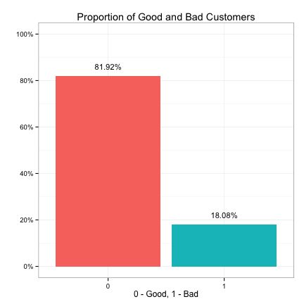
We see that ~82% of the customers in the upl dataset are good while ~18% are bad. This imbalanced distribution of the target variable implies that we can’t merely use the overall classification accuracy to measure model performance. For example, suppose we build a model, and it gives us an accuracy of 82%. We wouldn’t consider it good here because we can achieve the same 82% accuracy without fitting any model. Just simply guess every customer is good. Because we want to build models that can correctly identify the bad customers, we really need to use more granular measures such as sensitivity and specificity to measure model performance.

Having looked at the target variable, now let’s turn our attention to the predictors. We need to change the binary predictors to factors. But first, we change them to characters.

Next, we check which predictors have missing values.

We see purpose has more than 15% of its values missing, and market_value, debt_to_income and bankruptcy all have mild missings. Let’s explore the relationship between the target variable and the missing values.

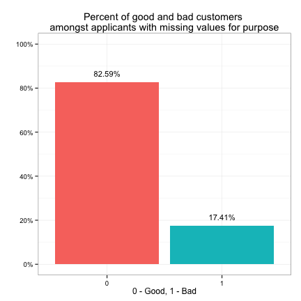
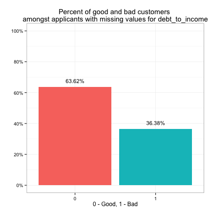
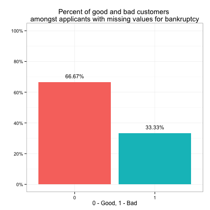
We see the target variable has the same distribution (82% good - 18% bad) amongst customers with missing purpose as amongst all customers. This is also true for market_value. This implies that we may choose to ignore the missing values when looking at the individual effect of purpose or market_value on the target variable. However, the target has a distribution of 67% good vs. 33% bad amongst customers with missing bankruptcy info, which is different from its overall distribution. The same is true for debt_to_income. This implies that we may not ignore the effect of missing values in bankruptcy or debt_to_income on the target.

Let’s perform the following missing value treatments. For purpose and bankruptcy, because they are categorical, we change their missing values to “unkown”. For debt_to_income, because it’s continuous, we fill its missing values with the median of its non-missing values. For market_value, because it is related with own_property, we first fill its missing values based on the values of own_property. In particular, for customers with own_property = 0, we fill their missing market values with zeros. For customers with own_property = 1, we fill their missing market values with the median of the non-missing values. Note that we use median instead of mean. This is because a few large values in market_value will result a big mean, while the median is more immune to outliers’ influence, and hence is a better measure of average in this case.

Now there’s no missing values in the data set. We can change the predictors from the character to factors

Finally, let’s create a data subfolder under proj_path and save the cleaned data there. We’ll use this cleaned data for descriptive analysis in the next section.

2.2 Descriptive Analysis

First, let’s load the cleaned data.

Next, let’s explore the relationships between the categorical predictors and the target. Because the target is binary (bad vs. good), we only need to look at how bad customers are distributed across the different levels of a given categorical predictor. We first create a helper function that takes a categorical predictor as an input parameter and calculates the percent of bad customers for each of its levels.

Here’s an example of how to use it.

Now we can draw bar chart to display these percentages of bad customers.

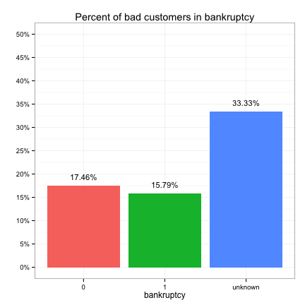
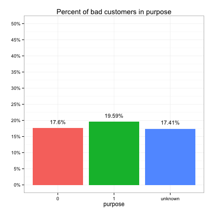
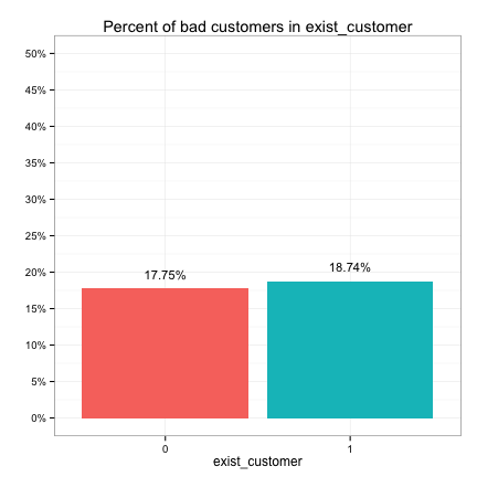
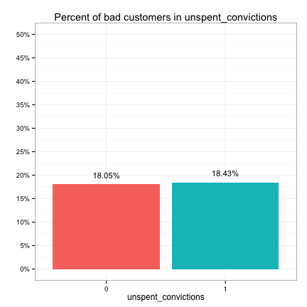
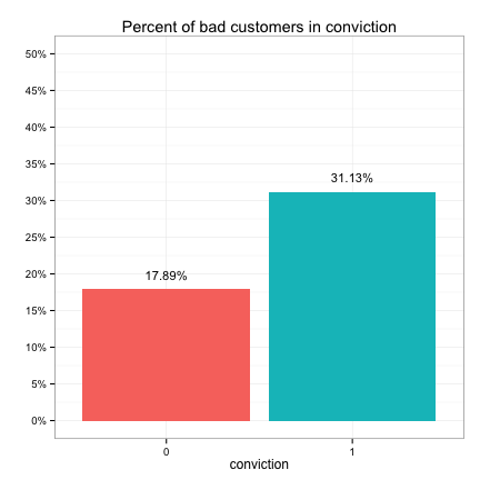
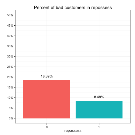
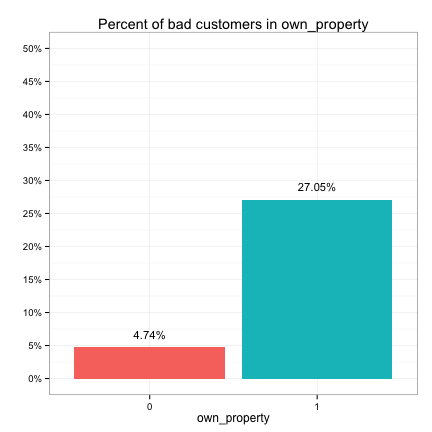
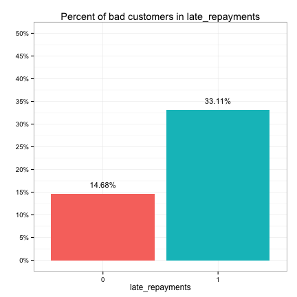
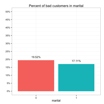
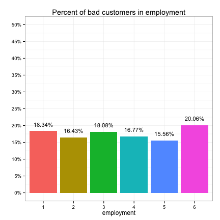
These plots suggest that the categorical predictors can be classified into three groups in terms of their potential predictive power:

• Strong: bankruptcy, conviction, repossess, own_property, late_repayments
• Weak: purpose, marital, employment
• None: exist_customer, unspent_convictions

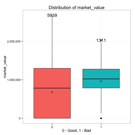
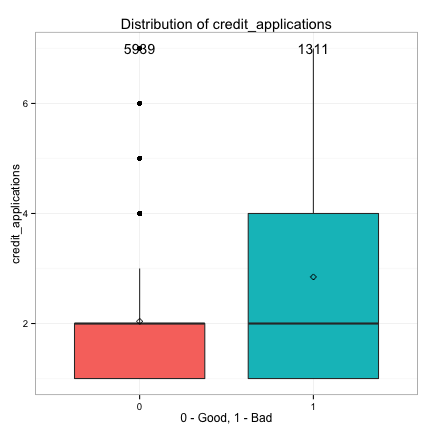
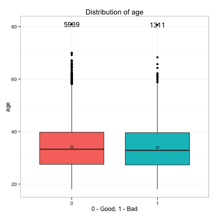
We also examine the relationships between the continuous predictors and the target.

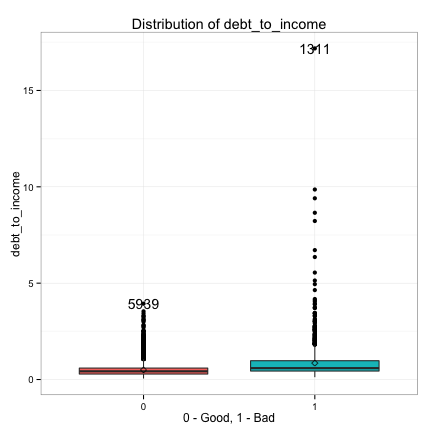
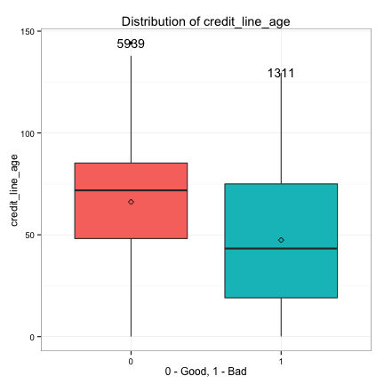
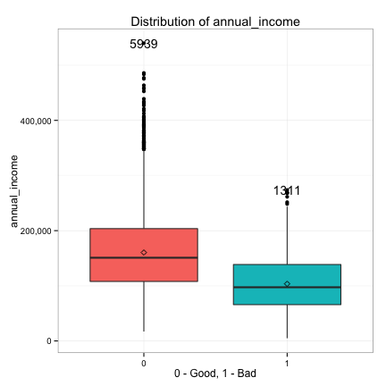
We see the distributions of debt_to_income and annual_income are heavily right skewed, so we take the log transform of debt_to_income and annual_income and replot.

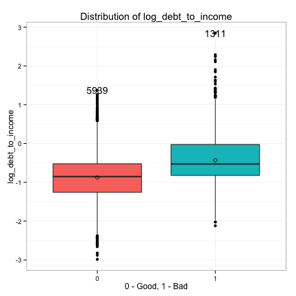
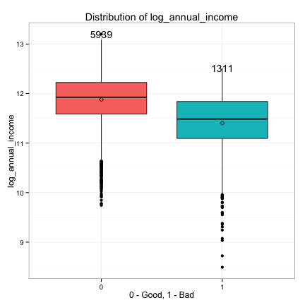
These plots suggest that the continuous predictors can also be classified into three groups in terms of their potential predictive power:

• Strong: log_debt_to_income, log_annual_income, credit_line_age
• Weak: market_value, credit_applications
• None: age

We also observe that the bulk of zero market values belong to the good customers, while only a few bad customers have zero market values. This suggests owning property (market value > 0) is possibly a strong predictor of a bad customer, which we already discovered when looking at the distribution of own_property just a moment ago. Therefore, it’s a good idea to create a categorical version of market_value by binning its values into different intervals based on its distribution.

We then plot the distribution of bad customers in market_value_cat.

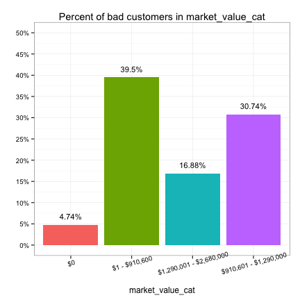
We see that market_value_cat is potentially a strong predictor. We’ll use it instead of market_value.

Finally, we collect the predictors into strong, weak and none groups as above discussed so that we can easily access them for future analysis.