Multiple Temperature Measurements
This project will measure the temperature at multiple points using DS18B20 sensors. We will use the waterproof version of the sensors since they are more practical for external applications.
The DS18B20 Sensor
The DS18B20 is a ‘1-Wire’ digital temperature sensor manufactured by Maxim Integrated Products Inc. It provides a 9-bit to 12-bit precision, Celsius temperature measurement and incorporates an alarm function with user-programmable upper and lower trigger points.
Its temperature range is between -55C to 125C and they are accurate to +/- 0.5C between -10C and +85C.
It is called a ‘1-Wire’ device as it can operate over a single wire bus thanks to each sensor having a unique 64-bit serial code that can identify each device.
While the DS18B20 comes in a TO-92 package, it is also available in a waterproof, stainless steel package that is pre-wired and therefore slightly easier to use in conditions that require a degree of protection. The measurement project that we will undertake will use the waterproof version.
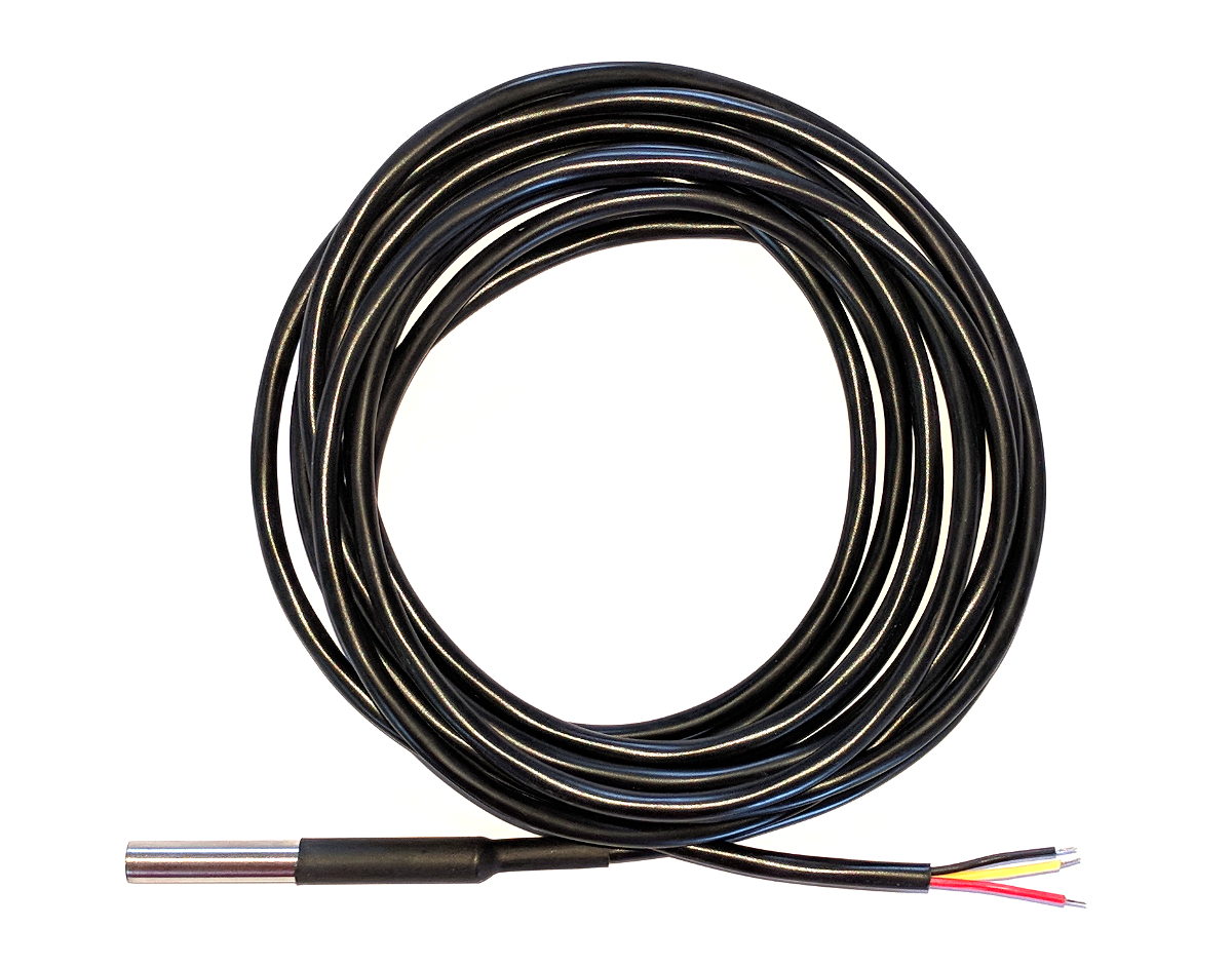
The sensors can come with a couple of different wire colour combinations. They will typically have a black wire that needs to be connected to ground. A red wire that should be connected to a voltage source (in our case a 3.3V pin from the Pi) and a blue or yellow wire that carries the signal.
The DS18B20 can be powered from the signal line, but in our project we will use an external voltage supply (from the Pi).
Measure
Hardware required
- 3 x DS18B20 sensors (the waterproof version)
- 10k Ohm resister
- Jumper cables with Dupont connectors on the end
- Solder
- Heat-shrink
Connect
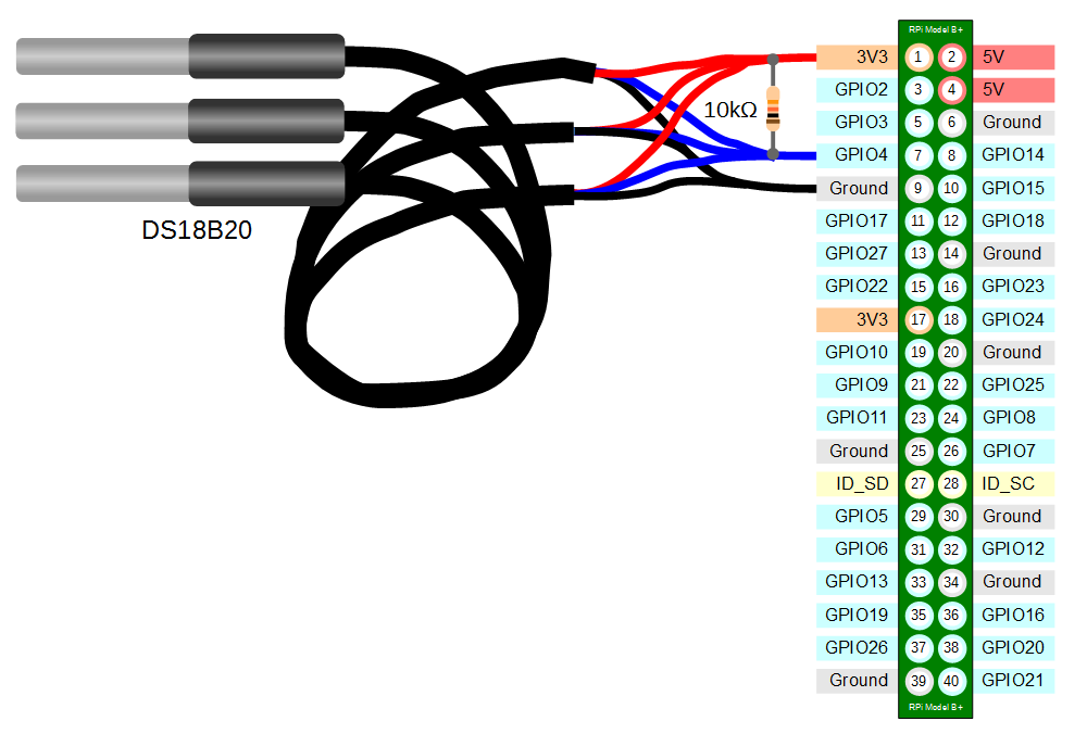
The DS18B20 sensors needs to be connected with the black wires to ground, the red wires to the 3V3 pin and the blue or yellow (some sensors have blue and some have yellow) wires to the GPIO4 pin. A resistor between the value of 4.7k Ohms to 10k Ohms needs to be connected between the 3V3 and GPIO4 pins to act as a ‘pull-up’ resistor.
The Raspbian Operating System image that we are using only supports GPIO4 as a 1-Wire pin, so we need to ensure that this is the pin that we use for connecting our temperature sensor.
The following diagram is a simplified view of the connection.
Connecting the sensor practically can be achieved in a number of ways. You could use a Pi Cobbler break out connector mounted on a bread board connected to the GPIO pins. But because the connection is relatively simple we could build a minimal configuration that will plug directly onto the appropriate GPIO pins using Dupont connectors. The resister is concealed under the heat-shrink and indicated with the arrow.

This version uses a recovered header connector from a computers internal USB cable.
Enable
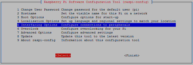
We’re going to go back to the Raspberry Pi Software Configuration Tool as we need to enable the 1-wire option. This can be done by running the following command;
Select ‘Interfacing options`;
Then select the 1-wire option and enable it.
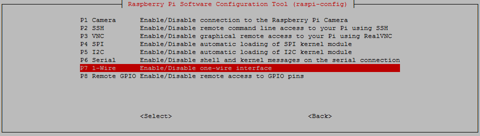
When you back out of the menu you will be asked to reboot the device. Do this and then log in again.
Test
From the terminal as the ‘pi’ user run the command;
modprobe w1-gpio registers the new sensors connected to GPIO4 so that now the Raspberry Pi knows that there is a 1-Wire device connected to the GPIO connector (For more information on the modprobe command check out the details here).
Then run the command;
modprobe w1-therm tells the Raspberry Pi to add the ability to measure temperature on the 1-Wire system.
To allow the w1_gpio and w1_therm modules to load automatically at boot we can edit the the /etc/modules file and include both modules there where they will be started when the Pi boots up. To do this edit the /etc/modules file;
Add in the w1_gpio and w1_therm modules so that the file looks like the following;
# /etc/modules: kernel modules to load at boot time.
#
# This file contains the names of kernel modules that should be loaded
# at boot time, one per line. Lines beginning with "#" are ignored.

w1-gpio
w1-therm
Save the file.
Then we change into the /sys/bus/w1/devices directory and list the contents using the following commands;
(For more information on the cd command check out the reference here. Or to find out more about the ls command go here)
This should list out the contents of the /sys/bus/w1/devices which should include a number of directories starting 28-. The number of directories should match the number of connected sensors. The portion of the name following the 28- is the unique serial number of each of the sensors.
We then change into one of those directories;
We are then going to view the ‘w1_slave’ file with the cat command using;
The output should look something like the following;
At the end of the first line we see a YES for a successful CRC check (CRC stands for Cyclic Redundancy Check, a good sign that things are going well). If we get a response like NO or FALSE or ERROR, it will be an indication that there is some kind of problem that needs addressing. Check the circuit connections and start troubleshooting.
At the end of the second line we can now find the current temperature. The t=23187 is an indication that the temperature is 23.187 degrees Celsius (we need to divide the reported value by 1000).
cd into each of the 28-xxxx directories in turn and run the cat w1_slave command to check that each is operating correctly. It may be useful at this stage to label the individual sensors with their unique serial numbers to make it easy to identify them correctly later.
Record
To record this data we will use a Python program that checks all the sensors and writes the temperature, sensor name and time into our database.
But first we need to ensure that our default version of Python running on the Pi is Python 3.
We can check what version is running by executing the following command;
If that indicates python 2.x, then we need to change that;
To find out what versions of Python 3 is available run the following
Hopefully you will see a 3.x version.
To change the default python version system-wide we can use the update-alternatives command. First list all available python alternatives;
There is a good chance that the output will be something like;
The above error message means that no python alternatives have been recognised by the update-alternatives command. For this reason we need to update our alternatives table and include both python 2 and 3 (make sure that you use the version numbers that are available on your system).
The last number on each of the previous lines is the priority, with the higher number being the highest priority
We can check again by running;
Our Python program will execute the program at a regular interval using cron which we used earlier to automatically reconnect to the network if required.
Record the temperature values
The following Python code (which is based on the code that is part of the great temperature sensing tutorial on iot-project) is a script which allows us to check the temperature reading from multiple sensors and write them to our database with a separate entry for each sensor.
The full code can be found in the code samples bundled with this book (m_temp.py).
#!/usr/bin/python
# -*- coding: utf-8 -*-

import os
import fnmatch
import time
import sqlite3            #Import SQLite library
import logging

logging.basicConfig(filename='/home/pi/DS18B20_error.log',
  level=logging.DEBUG,
  format='%(asctime)s %(levelname)s %(name)s %(message)s')
logger=logging.getLogger(__name__)

# Load the modules (not required if they are loaded at boot)
# os.system('modprobe w1-gpio')
# os.system('modprobe w1-therm')

# Get the time in the right format
dtg = time.strftime('%Y-%m-%d %H:%M:%S', time.localtime())

temperature = []
IDs = []

# Function for storing readings into the database
def insertDB(IDs, temperature, dtg):
  try:
    # Opens a file called measurements
    db = sqlite3.connect('/home/pi/measurements')
    # Get a cursor object
    cursor = db.cursor()
    # Insers the values into the table
    for i in range(0,len(temperature)):
      cursor.execute('''INSERT INTO temperature( \
                        dtg, temperature, sensor_id)
                        VALUES(?,?,?)''', (dtg, temperature[i], IDs[i]))

      # Commit the change
      db.commit()
  # Catch any exception
  except Exception as e:
    # Roll back any change if something goes horribly wrong
    db.rollback()
    raise e
  finally:
    # Close the db connection
    db.close()

for filename in os.listdir("/sys/bus/w1/devices"):
  if fnmatch.fnmatch(filename, '28-*'):
    with open("/sys/bus/w1/devices/" + filename + "/w1_slave") as f_obj:
      lines = f_obj.readlines()
      if lines[0].find("YES"):
        pok = lines[1].find('=')
        temperature.append(float(lines[1][pok+1:pok+6])/1000)
        IDs.append(filename)
      else:
        logger.error("Error reading sensor with ID: %s" % (filename))

if (len(temperature)>0):
  insertDB(IDs, temperature, dtg)
This script can be saved in our home directory (/home/pi) and can be run by typing;
Run this script a few times and then we can check the results in our database by starting up SQLite as follows;
From the SQLite prompt we can query the database to return all the records using SELECT * FROM temperature; as follows;
There are three records for each time that we ran the program, including the times they were taken, the temperature recorded and the serial number of the sensor.
Recording data on a regular basis with cron
As mentioned earlier, while our code is a thing of beauty, it only records a single entry for the light every time it is run.
What we need to implement is a schedule so that at a regular time, the program is run. This is achieved using cron via the crontab.
To set up our schedule we need to edit the crontab file. This is is done using the following command;
Once run it will open the crontab in the nano editor. We want to add in an entry at the end of the file that looks like the following;
This instructs the computer that every minute of every hour of every day of every month we run the command /usr/bin/python /home/pi/m_temp.py (which, if we were at the command line in the pi home directory, we would run as python m_temp.py, but since we can’t guarantee where we will be when running the script, we are supplying the full path to the python command and the m_temp.py script.
Save the file and when the next minute rolls over our program will run on its designated schedule and we will have sensor entries written to our database every minute. Go ahead, check it out by refreshing the temperature table.
Managing database size
While it’s a great idea to save our local data into a database, we stand the risk of gradually letting that database fill up until it exceeds the capacity of our storage.
In the case of the measurements that we are carrying out, the readings are happening pretty regularly, so it’s worth thinking about. Capturing some simple measurements every minute means in the scheme of things that’s about 30,000 recordings per week.
What we’re looking for is a script that will run on a repeating schedule and remove old records. Sound familiar? That’s a very similar process to what we are doing when we record our data. A python script that is executed regularly by cron.
Here’s how we can do it.
The following python script (which we can name db-manage.py) opens our database, deletes any records older than a year, cleans up and exits.
#!/usr/bin/python
#encoding:utf-8

#Import SQLite library
import sqlite3

# Opens a database file called measurements
conn = sqlite3.connect('/home/pi/measurements', isolation_level=None)
db = conn.cursor()

# Delete any records that are older than 1 year
db.execute('DELETE FROM temperature WHERE dtg<DATETIME("now","localtime", "-1 yea\
rs")')
# VACUUM the database to remove any unnecessary data
db.execute('VACUUM')

# Commit the changes to the database and close the connection
conn.commit()
conn.close
The file is available as db-manage.py and can be found in the code sample extras that can be downloaded with this book.
It’s a pretty simple script and we can schedule its operation by editing the crontab file like so;
We want to add in an entry at the end of the file that looks like the following;
1 0 */1 * * /usr/bin/python /home/pi/db-manage.py
This instructs the computer that at 1 minute past the hour at midnight (hence the 0) on the 1st day of every month we run the command /usr/bin/python /home/pi/db-manage.py (which, if we were at the command line in the pi home directory, we would run as python db-manage.py, but since we can’t guarantee where we will be when running the script, we are supplying the full path to the python command and the db-manage.py script.
Save the file and every month our program will run on its designated schedule and will make sure to delete any records older than a year.
Explore
Simple data point API
The main mechanism for exploring and using our data is going to be via a simple data block returned from a http request.
What does all that actually mean?
That’s a good question. Ultimately we’re measuring something and we want to be able to communicate that measurement to an external service. That service could be another database somewhere or to a web page or to a system that will alert based on the value of the light levels being within certain boundaries.
The very simplest way that we can do this is to present the data as the measured values when we ask for them in a web request. This could be thought of as a simplified form of an API (and I plan to make something more complicated in the future).
The data will be presented as JSON as that is one of the most ubiquitous data forms around.
Enough esoterica, what does the magic code look like that will do this?
<?php

$db = new PDO('sqlite://home/pi/measurements');

$result = $db->query('SELECT * FROM temperature ORDER BY dtg DESC LIMIT 1');

$datapie = array();

$result->setFetchMode(PDO::FETCH_ASSOC);

while ($row = $result->fetch()) {
    extract($row);
    echo json_encode($row);
}

?>
We can save this file as temperature.php and have it in the /var/www/html directory on our Pi (temperature.php can be found in the code sample extras that can be downloaded with this book).
How we can put in the IP address of our Pi to our browser along with our distance php file (http://10.1.1.160/temperature.php) and we should get something like the following appear in the browser;
What good will getting this data be? Well……. I’m a bit of a believer that the information that gets captured by the Pi shouldn’t ultimately reside on the device in the long term. In the perfect world I would see it being requested by an external service that was checking a range of data points that would exist around the home (pressure, temperature inside / outside, CO2 levels, is the car parked in the garage, that sort of thing) so this is more of an enabling device than a ‘let’s display stuff’ deal. But I hear what you’re saying. “That’s lame. How can I impress people with that?”. Fair point. To deal with that problem let’s make a simple graph.
Extracting a Range of Data
Righto… If we’re going to make a graph of our light levels we’ll need a variation of our API that will gather and present a range of data that our graph can then display.
This will form a piece of code that our graph will use as a JSON formatted data source.
It will look as follows;
<?php

$data= array();

// connect to the database
$db = new PDO("sqlite://home/pi/measurements");
$db->setAttribute(PDO::ATTR_ERRMODE, PDO::ERRMODE_EXCEPTION);

// prepare SQL command and execute
$query = "SELECT * FROM light WHERE
          dtg>DATETIME('now','localtime', '-24 hours')";
$result = $db->prepare( $query );
$result->execute();

// compile the returned data
$values = $result->fetchAll(PDO::FETCH_ASSOC);
array_push($data, $values);

// print the data
echo json_encode($values);

// close the database connection
$db = NULL;

?>
This block of PHP code will connect to our database and instead of returning a single piece of data it will return (‘echo’) a range of values from the past 24 hours. We’ll call the file temperature-range.php and it will be in the /var/www/html directory. A copy of the file can be found in the code sample extras that can be downloaded with this book.
Graphing Our Data
The following file is our graph which will use our temperature-range.php file and display it. It uses the d3.js visualisation library and for a full description of the workings of the code please feel free to consult a copy of ‘D3 Tips and Tricks v6.x’. It’s free and can be downloaded from here.
<!DOCTYPE html>
<meta charset="utf-8">
<style> /* set the CSS */

body { font: 12px Arial;}

path {
    stroke: steelblue;
    stroke-width: 2;
    fill: none;
}

.axis path,
.axis line {
    fill: none;
    stroke: grey;
    stroke-width: 1;
    shape-rendering: crispEdges;
}

.legend {
    font-size: 16px;
    font-weight: bold;
    text-anchor: middle;
}

</style>
<body>

<!-- load the d3.js library -->
<script src="https://d3js.org/d3.v6.min.js"></script>

<script>

// Set the dimensions of the canvas / graph
var margin = {top: 30, right: 20, bottom: 70, left: 50},
    width = 900 - margin.left - margin.right,
    height = 300 - margin.top - margin.bottom;

// Parse the date / time
var parseDate = d3.timeParse("%Y-%m-%d %H:%M:%S");

// Set the ranges
var x = d3.scaleTime().range([0, width]);
var y = d3.scaleLinear().range([height, 0]);

// Define the line
var priceline = d3.line()
    .x(function(d) { return x(d.date); })
    .y(function(d) { return y(d.price); });

// Adds the svg canvas
var svg = d3.select("body")
    .append("svg")
        .attr("width", width + margin.left + margin.right)
        .attr("height", height + margin.top + margin.bottom)
    .append("g")
        .attr("transform",
              "translate(" + margin.left + "," + margin.top + ")");

// Get the data
d3.json("temperature-range.php").then(function(data) {

  data.forEach(function(d) {
		d.date = parseDate(d.dtg);
		d.price = +d.temperature;
		d.symbol = d.sensor_id;
    });

    // Scale the range of the data
    x.domain(d3.extent(data, function(d) { return d.date; }));
    y.domain(d3.extent(data, function(d) { return d.price; }));

    // Group the entries by symbol
    dataNest = Array.from(
	    d3.group(data, d => d.symbol), ([key, value]) => ({key, value})
	  );

    // set the colour scale
    var color = d3.scaleOrdinal(d3.schemeCategory10);

    legendSpace = width/dataNest.length; // spacing for the legend

    // Loop through each symbol / key
    dataNest.forEach(function(d,i) {

        svg.append("path")
            .attr("class", "line")
            .style("stroke", function() { // Add the colours dynamically
                return d.color = color(d.key); })
            .attr("id", 'tag'+d.key.replace(/\s+/g, '')) // assign an ID
            .attr("d", priceline(d.value));

        // Add the Legend
        svg.append("text")
            .attr("x", (legendSpace/2)+i*legendSpace)  // space legend
            .attr("y", height + (margin.bottom/2)+ 5)
            .attr("class", "legend")    // style the legend
            .style("fill", function() { // Add the colours dynamically
                return d.color = color(d.key); })
            .on("click", function(){
                // Determine if current line is visible
                var active   = d.active ? false : true,
                newOpacity = active ? 0 : 1;
                // Hide or show the elements based on the ID
                d3.select("#tag"+d.key.replace(/\s+/g, ''))
                    .transition().duration(100)
                    .style("opacity", newOpacity);
                // Update whether or not the elements are active
                d.active = active;
                })
            .text(
                function() {
		            if (d.key == '28-00043b6ef8ff') {return "Inlet";}
		            if (d.key == '28-00043e9049ff') {return "Ambient";}
		            if (d.key == '28-00043e8defff') {return "Outlet";}
		            else {return d.key;}
		            });

    });

  // Add the X Axis
  svg.append("g")
      .attr("class", "axis")
      .attr("transform", "translate(0," + height + ")")
      .call(d3.axisBottom(x));

  // Add the Y Axis
  svg.append("g")
      .attr("class", "axis")
      .call(d3.axisLeft(y));

});

</script>
</body>
We will want to place a copy of this file which we will call temperatures-graph.html in the /var/www/html directory. A copy of it can be found in the code sample extras that can be downloaded with this book.
We can see the end result by putting the web address into our browser. It should look something like http://10.1.1.160/temperatures-graph.html. The end result should look a bit like the following (depending on the number of sensors you are using, and the amount of data you have collected)
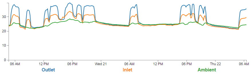
One of the neat things about this graph is that it ‘builds itself’ in the sense that aside from us deciding what we want to label the specific temperature streams as, the code will organise all the colours and labels for us. Likewise, if the display is getting a bit messy we can click on the legend labels to show / hide the corresponding line.
Wrap Up
We’ve assembled our Raspberry Pi with temperature sensors. We installed an operating system and configured it for use. We’ve set up networking and installed a database and a web server. We’ve written code to record data into our database and an API to pull data out of it. We’ve even installed a graph to display it in a visual form. Nice work.
There is a strong possibility that the information I have laid out here could be littered with evil practices and gross inaccuracies.
But look on the bright side. Irrespective of the nastiness of the way that any of it was accomplished or the inelegance of the code, if the picture drawn on the screen is relatively pretty, you can walk away with a smile. :-)
Those with a smattering of knowledge of any of the topics I have butchered above (or below) are fully justified in feeling a large degree of righteous indignation. To those I say, please feel free to amend where practical and possible, but please bear in mind this was written from the point of view of someone with only a little experience in the topic and therefore try to keep any instructions at a level where a new entrant can step in.