6. Valuing European and American options
I have written about option pricing earlier. The introduction to option pricing gave an overview of the theory behind option pricing. The post on introduction to binomial trees outlined the binomial tree method to price options.
In this post, we will use QuantLib and the Python extension to illustrate a simple example. Here we are going to price a European option using the Black-Scholes-Merton formula. We will price them again using the Binomial tree and understand the agreement between the two.
In [1]: import QuantLib as ql
        import utils
        %matplotlib inline
European Option
Let us consider a European call option for AAPL with a strike price of 130 maturing on 15th Jan, 2016. Let the spot price be 127.62. The volatility of the underlying stock is know to be 20%, and has a dividend yield of 1.63%. Let’s value this option as of 8th May, 2015.
In [2]: maturity_date = ql.Date(15, 1, 2016)
        spot_price = 127.62
        strike_price = 130
        volatility = 0.20 # the historical vols for a year
        dividend_rate =  0.0163
        option_type = ql.Option.Call

        risk_free_rate = 0.001
        day_count = ql.Actual365Fixed()
        calendar = ql.UnitedStates(ql.UnitedStates.GovernmentBond)

        calculation_date = ql.Date(8, 5, 2015)
        ql.Settings.instance().evaluationDate = calculation_date
We construct the European option here.
In [3]: payoff = ql.PlainVanillaPayoff(option_type, strike_price)
        exercise = ql.EuropeanExercise(maturity_date)
        european_option = ql.VanillaOption(payoff, exercise)
The Black-Scholes-Merton process is constructed here.
In [4]: spot_handle = ql.QuoteHandle(
            ql.SimpleQuote(spot_price)
        )
        flat_ts = ql.YieldTermStructureHandle(
            ql.FlatForward(calculation_date,
                           risk_free_rate,
                           day_count)
        )
        dividend_yield = ql.YieldTermStructureHandle(
            ql.FlatForward(calculation_date,
                           dividend_rate,
                           day_count)
        )
        flat_vol_ts = ql.BlackVolTermStructureHandle(
            ql.BlackConstantVol(calculation_date,
                                calendar,
                                volatility,
                                day_count)
        )
        bsm_process = ql.BlackScholesMertonProcess(spot_handle,
                                                   dividend_yield,
                                                   flat_ts,
                                                   flat_vol_ts)
Lets compute the theoretical price using the AnalyticEuropeanEngine.
In [5]: european_option.setPricingEngine(ql.AnalyticEuropeanEngine(bsm_process))
        bs_price = european_option.NPV()
        print("The theoretical price is %lf" % bs_price)

Out[5]: The theoretical price is 6.749272
Lets compute the price using the binomial-tree approach.
In [6]: def binomial_price(option, bsm_process, steps):
            binomial_engine = ql.BinomialVanillaEngine(bsm_process, "crr", steps)
            option.setPricingEngine(binomial_engine)
            return option.NPV()

        steps = range(2, 200, 1)
        prices = [binomial_price(european_option, bsm_process, step) for step in step\
s]
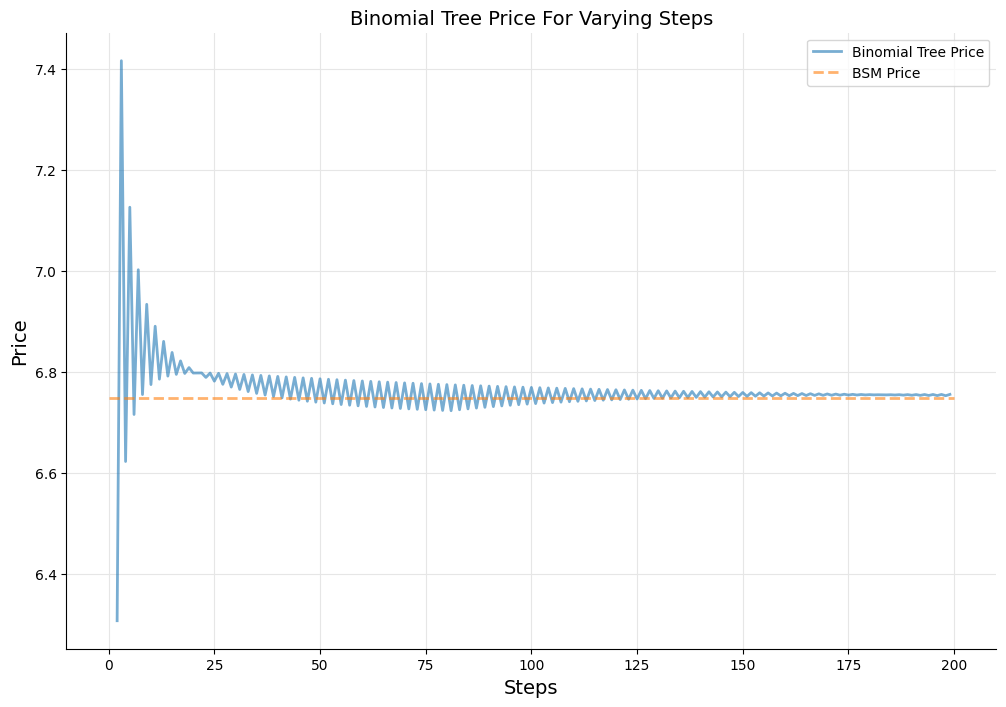
In the plot below, we show the convergence of binomial-tree approach by comparing its price with the BSM price.
In [7]: fig, ax = utils.plot()
        ax.plot(steps, prices, label="Binomial Tree Price", lw=2, alpha=0.6)
        ax.plot([0,200],[bs_price, bs_price], "--", label="BSM Price", lw=2, alpha=0.\
6)
        ax.set_xlabel("Steps", size=14)
        ax.set_ylabel("Price", size=14)
        ax.set_title("Binomial Tree Price For Varying Steps", size=14)
        ax.legend();
American Option
The above exercise was pedagogical, and introduces one to pricing using the binomial tree approach and compared with Black-Scholes. As a next step, we will use the Binomial pricing to value American options.
The construction of an American option is similar to the construction of European option discussed above. The one main difference is the use of AmericanExercise instead of EuropeanExercise use above.
In [8]: payoff = ql.PlainVanillaPayoff(option_type, strike_price)
        settlement = calculation_date
        am_exercise = ql.AmericanExercise(settlement, maturity_date)
        american_option = ql.VanillaOption(payoff, am_exercise)
Once we have constructed the american_option object, we can price them using the Binomial trees as done above. We use the same function we constructed above.
In [9]: steps = range(2, 200, 1)
        prices = [binomial_price(american_option, bsm_process, step) for step in step\
s]

In [10]: fig, ax = utils.plot()
         ax.plot(steps, prices, label="Binomial Tree Price", lw=2, alpha=0.6)
         ax.plot([0,200],[bs_price, bs_price], "--", label="BSM Price", lw=2, alpha=0\
.6)
         ax.set_xlabel("Steps", size=14)
         ax.set_ylabel("Price", size=14)
         ax.set_title("Binomial Tree Price For Varying Steps", size=14)
         ax.legend();
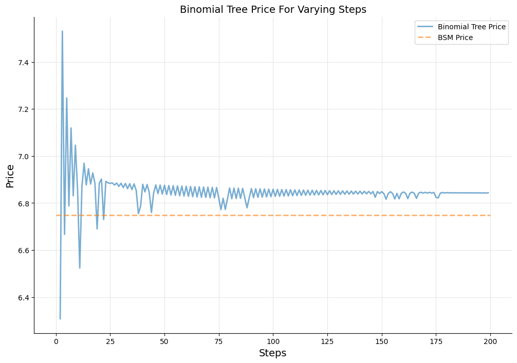
Above, we plot the price of the American option as a function of steps used in the binomial tree, and compare with that of the Black-Scholes price for the European option with all other variables remaining the same. The binomial tree converges as the number of steps used in pricing increases. American option is valued more than the European BSM price because of the fact that it can be exercised anytime during the course of the option.
Conclusion
In this chapter we learnt about valuing European and American options using the binomial tree method.