2 Machine Learning
Deep learning is a family of techniques for building predictive models that are at the center of the current boom in “artificial intelligence”. In the past decade deep learning models have been able to surpass “traditional” techniques in many domains and applications, sometimes even exceeding human performance. But to understand deep learning, we need to put it in the larger context of machine learning, as deep learning is itself one type of machine learning. We will also look at shallow neural networks, the ancestors of deep learning.
In this chapter and the next we’ll go over some of the core concepts of machine learning and the basics of neural networks, setting us up to learn about modern, deep neural networks.
What is machine learning?
Machine learning (ML) is an approach to solving problems, where data is used directly to adjust the internal parameters of a computer program to provide the best answers possible. Examples include predicting the ultimate sale price of a house or detecting the presence of a tumor in a medical scan. The difference between machine learning programs (usually called “models”) and traditional computer programs is that instead of having programmers explicitly write the logic of the program by hand, the important decision logic is “learned” by the program by looking at example data. This process is called training the model.
Machine learning is closely related to (and sometimes identical to) statistical modeling. The main differences are in the historical development and the emphasis on outcomes and explanatory power. Machine learning tends to focus on producing the most highly predictive models, even if they are effectively “black boxes”1 to the users. Statistical modeling has more emphasis on creating models that have more explanatory power (e.g. creating a model that mimics the underlying process that generates the data). Statistics has also built out robust techniques to deal with small amounts of data, which many practitioners of ML tend to avoid. That said, there are many concepts from statistics that underlie ML and deep learning.
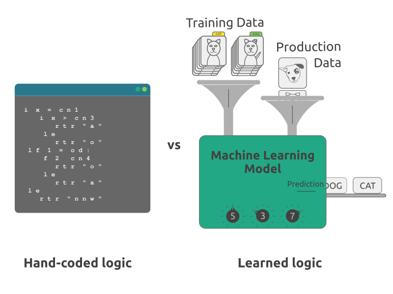
As more data has become available in many areas of science, industry, and government, machine learning has been increasingly adopted as a viable solution to solve real-world problems. The abundance of data is however not the only factor. More data plus cheaper storage and computing power has led to the development of more software (especially open source software) and the refinement of techniques to make the best use of that data. This has been especially true of deep learning, as we will see in later chapters.
Types of machine learning tasks and solutions
Most problems that machine learning is used to solve can be thought of as predictions problems. Some fit more into the casual usage of the term “prediction”, as in predicting the ultimate sale price of a house, which will only be known at some point in the future. Others are predictions in a technical sense, such as predicting whether a certain image is of a dog or a cat.
Regression
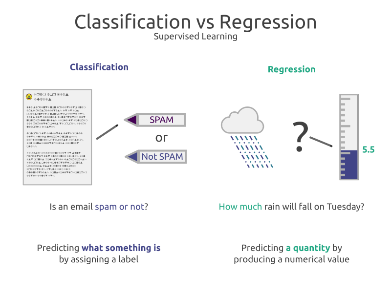
Machine learning tasks can be broken down into a handful of categories. A common way to categorize tasks is by the type of output that a machine learning model needs to produce. One of the most common types of task is regression2. Regression is the task of predicting a (continuous) numerical value, such as the temperature in a weather forecast, the sales volume of a product, or estimating time of arrival of a vehicle.
The most basic version of regression that many people are familiar with is finding the slope and intercept of a “best fit line” that fits some data points. This line can then be used to predict other values by using the basic line equation to estimate new, unseen values. This is the manual version of finding the best fit slope and intercept values (a.k.a. parameters). In ML, as we’ll discuss in more detail, those slope and intercept parameters are determined by the training process, where different values are tried iteratively and the fit of the line is compared with the known data to see how good the fit is. This is the core of machine learning: “learning” the best parameter values of a model from the known, existing data.
Regression is one of the most common applications of machine learning and typically falls under the category of supervised learning, which we will discuss below.
Classification
Classification is the task of predicting the class, category, or label of an item. This can be a task with many possible choices, such as facial recognition, or a binary, yes/no scenario, such as predicting whether a customer will purchase an advertized item. Other examples include predicting the species of an animal present in an image, the sentiment of a product review, whether a self-driving car needs to make an emergency stop, and how a support request should be routed.
A simple classification algorithm is the flow chart, which is similar to the decision tree. A medical doctor might create a flow chart to map out how to make a certain medical diagnosis based on symptoms, medical history, and measured patient data. The doctor does this based on their knowledge and understanding of how they make decisions based on the available data. The doctor creates decision criteria for each piece of input data, such as body temperature. The path of the flow chart, based on each decision, leads to the medical diagnosis, or “classification”. A similar model can be created with machine learning. Instead of the doctor manually inputting the decision thresholds and the overall flow of the decisions, the decision criteria are learned from the available data by trying out many combinations of decision thresholds and structures and evaluating the overall goodness of the predictions, until the best decision thresholds and flow structure are found.
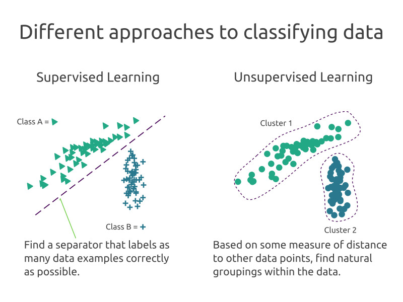
As with regression, classification tasks typically fall under the umbrella of supervised learning. Sometimes you don’t know what the classes are for a classification problem, so instead you try to discover clusters or groupings in the data based on similarities. This is unsupervised learning, which we will discuss below.
Supervised learning
Another way to organize machine learning tasks is by the method used to solve the problem, rather than the type of predictive task. One of the most common classes of methods used to build predictive models is “supervised learning”. Supervised learning is when you have data to train a model that includes “ground truth” answers. For example, if you were building a model to predict how tall children would be as adults, you could use a supervised learning approach if you had data on full-grown adults when they were children and their final, adult heights. The inputs to the model would be the earlier data, such as age, height, height of parents, etc, and the matching outputs would be the known, final heights of those people.
Essentially supervised learning is when you train a model by taking example inputs and comparing the predictions of the model to the known, desired outputs. By altering the parameters of the model (think the slope and intercept of your fit line), you can then check if the new parameters provide an improvement in the overall predictive performance of the model. In practice this is done by training algorithms, which automatically try many possible model parameter values to land on the best model, given the current data.
Unsupervised learning
In contrast to supervised learning is “unsupervised learning”, where you do not have the “ground truth” answers for the task you are trying to address. One of the most common tasks using unsupervised learning is “clustering”. When clustering, you want to discover natural groupings of data, based on similarities within the data set. For example, you might want to cluster customers by purchasing behavior or demographic information to create focused advertising campaigns. You may not know what these groupings are beforehand or how many groups to expect. Only after investigating the members of these clusters can you (potentially) give them labels that make sense. This is in contrast to supervised learning, where you know beforehand how many classes you have and what they are. These additional challenges can make unsupervised learning more difficult to perform, but it may be worth it if collecting the “ground truth” is very costly or even impossible.
Self-supervised learning
There are some approaches to solving problems that use “unlabeled” data, but in a different way than the unsupervised approaches mentioned above. Instead of searching for natural clusters or patterns within the data, you can pose tasks where the answer is already contained in the data. Examples include training models to predict the next word in a sentence, using the first part of the sentence as the input and the following word(s) as the “ground truth” output, effectively formulating the task as a supervised learning problem. This reformulation from “unlabeled” data to a supervised learning problem is why the moniker “self-supervised” is used, as the data is its own label.
The distinction between supervised, unsupervised, and semi-supervised learning is not always clear-cut, but it is often a useful one3.
Reinforcement learning
Another category of machine learning is “reinforcement learning”. Reinforcement learning is an approach to solving tasks where a strategy for decision making is learned, typically trying to maximize or minimize some score or ultimate goal. Common examples of tasks that reinforcement learning is applied to are games, where the player needs to make a series of decisions, given the state of play. The reinforcement learning model may learn from the score in the game, winning or losing, or all of those combined. Reinforcement learning combined with deep learning has been used successfully in many gaming tasks in recent years4. Reinforcement learning will not be further covered in this book.
An example task
Before we look at the details of how machine learning problems are formulated and solutions are built and tested, let’s consider an example problem. This will give us even more context when we discuss the specifics of how machine learning solutions are created.
Predicting real estate sales prices
Let’s imagine that you decide that you want to buy some real estate (e.g. a house). You want to use your computing skills to give you the best understanding possible of how much to pay for a house by building a program that could predict how much a given house would ultimately sell for. How would you do this?
As we have seen above, this is a regression problem. We want to know a specific numerical estimate: the price in some currency. If you were a physicist, cough, you might try to build a model from first principles. One based on assumptions about how humans act and information about the fundamental attributes of the house. This probably won’t work, as the underlying mechanisms are far too complicated. The machine learning approach would be to try to use data to adjust a mathematical model, such that the model can effectively use the different characteristics of the house to predict the sales price. By collecting data from recent sales of homes in the region, you could use the known characteristics, or features, of these homes as training inputs to an ML model and compare the predicted sales prices to the known, actual sales prices.
Assuming you had selected a model and trained it using the data you had, how would you know if the model was good? A good model should produce price predictions that are close to the actual sales prices of homes in the area. While training, you would compare the outputs of your model to the known values, adjust the internal parameters of the model, check the overall goodness of the predictions, and iterate this process until the model is no longer improving or you are satisfied. This training process is done via a training algorithm, which is usually specific to the type of machine learning model you are training.
One immediate issue with this is that your model may be able to learn to predict the sales prices of the examples you have (effectively memorizing them), but, when faced with new data, not be able to make reasonable predictions. Your model has focused on memorizing the training data, rather than on learning the more general patterns that are useful for predicting sales prices of houses that it has not yet seen. The way to understand and quantify the goodness of your model is to test it on house sales data that it did not see during the training process. This will help estimate how it will do with “real world” data.
The basic steps in this example are:
- Formulate the problem
- Collect necessary data
- Train the model
- Evaluate the performance of the model
- Iterate as necessary
There are a lot of details that I have glossed over in this example of a supervised regression problem, but we have now set the stage to dive into those details more deeply.
Formulating machine learning problems
This content is not available in the sample book. The book can be purchased on Leanpub at http://leanpub.com/zefsguide2dl.
Data sets and features
This content is not available in the sample book. The book can be purchased on Leanpub at http://leanpub.com/zefsguide2dl.
Measuring performance
Probably the most important question about a machine learning model is how good the model is. This question sounds straight-forward, but how you measure the performance of a model is something that ML practitioners often must spend a lot of effort on.
For regression tasks, common measures of performance are the mean absolute error, MAE, and the root-mean-square error, RMSE. These quantify the typical error of predictions made by the model. Both look at the difference between a prediction and the “ground truth”, while treating an overestimate the same as an underestimate, but RMSE effectively “focuses” on large errors in a disproportionate way. This is often preferred, if large prediction errors are especially costly. In contrast to this, you might have a task where overestimation is fine, but underestimation is very costly, so using a symmetric metric, such as MAE or RMSE would not be appropriate and a “weighted” approach would be better suited.
Classification tasks have their own set of performance metrics and even more explicit tradeoffs, depending on the issues related to incorrect predictions. Common classification metrics include accuracy, precision, recall, specificity, and F1 score. We will discuss some of these in more detail when we talk about classification tasks for deep learning.
Regardless of the task, the most appropriate performance metric should be chosen, taking into account the pros and cons as relates to the specific task.
Performance baselines and success thresholds
One of the difficulties in trying to solve problems with machine learning is that large amounts of data and long training times are often needed before good performance levels are achieved. The practical drawback of this is that “starting small” and moving incrementally is often not feasible. That means that it’s common to dive in with what seems like a good idea, only to discover that the idea does not result in a good model after much effort.
One mitigation strategy is to establish performance baselines. By quantifying the performance of the current solution, you can set a baseline for how well the new model needs to perform. If there is no current solution, you can create a baseline solution by starting with something as simple as possible, such as using the mean price or a very simple linear model for predicting real estate prices. If your model does worse than that simple baseline, you know that you are on the wrong track5.
Along with performance baselines, it’s very important to establish success thresholds for models. How far off can your real estate sales price predictor be and still be considered good enough? $100, $1,000, $10,000? This is even more important when you are building models at the request of others who will ultimately rely on those models.
Model selection
This content is not available in the sample book. The book can be purchased on Leanpub at http://leanpub.com/zefsguide2dl.
Model training
This content is not available in the sample book. The book can be purchased on Leanpub at http://leanpub.com/zefsguide2dl.
Supervised learning
This content is not available in the sample book. The book can be purchased on Leanpub at http://leanpub.com/zefsguide2dl.
Splitting data sets for training
This content is not available in the sample book. The book can be purchased on Leanpub at http://leanpub.com/zefsguide2dl.
Unsupervised learning
This content is not available in the sample book. The book can be purchased on Leanpub at http://leanpub.com/zefsguide2dl.
Dimensionality reduction
This content is not available in the sample book. The book can be purchased on Leanpub at http://leanpub.com/zefsguide2dl.
Loss functions
This content is not available in the sample book. The book can be purchased on Leanpub at http://leanpub.com/zefsguide2dl.
Parameter optimization
This content is not available in the sample book. The book can be purchased on Leanpub at http://leanpub.com/zefsguide2dl.
Gradient descent
This content is not available in the sample book. The book can be purchased on Leanpub at http://leanpub.com/zefsguide2dl.
Generalization and overfitting
This content is not available in the sample book. The book can be purchased on Leanpub at http://leanpub.com/zefsguide2dl.
Bias and variance
Two of the most important ways to quantify how well a model behaves are bias and variance. In general you can think of bias as how consistently off an estimate is from the true value. More specific to ML, bias is how far off a model trained with a given set of hyperparameters is from the the true target value when being used to predict the target value from a test set. In other contexts this is called systematic error, rather than random error or noise. To characterize the bias, multiple estimates of a value need to be made. The mean error of those estimates is the bias.
For ML models, the bias is the mean error from multiple models all with the same hyperparameters, but trained on different samples of the training data. This estimates how far off (and in what direction) a specific model will be from the “ground truth”.
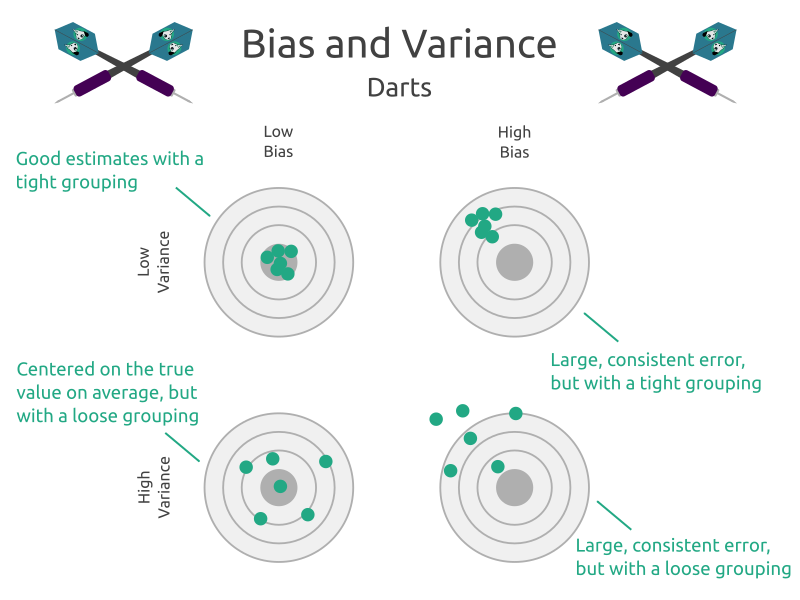
Variance is a measure of how “spread out” a set of values are. For ML models this is the spread of predictions for a single point in the test set, as made by several instances of the same model (i.e. same hyperparameters) trained on different samples of the training data. A model that overfits will result in several models that give widely varying predictions of the same input, as each model has learned the very specific patterns in the samples, rather than the more general pattern common to all samples.
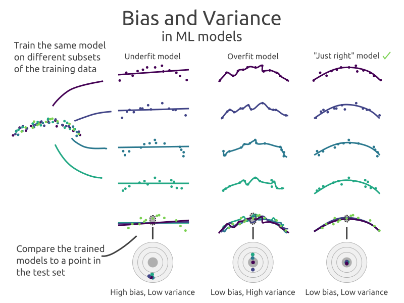
The ideal model has low bias and low variance. In practice there is typically a trade off between having either a low bias or low variance model and the best choice is a moderately low bias and moderately low variance model.
Avoiding overfitting
This content is not available in the sample book. The book can be purchased on Leanpub at http://leanpub.com/zefsguide2dl.
Regularization
This content is not available in the sample book. The book can be purchased on Leanpub at http://leanpub.com/zefsguide2dl.
Hyperparameters
This content is not available in the sample book. The book can be purchased on Leanpub at http://leanpub.com/zefsguide2dl.
Productionization
This content is not available in the sample book. The book can be purchased on Leanpub at http://leanpub.com/zefsguide2dl.
Common issues
This content is not available in the sample book. The book can be purchased on Leanpub at http://leanpub.com/zefsguide2dl.
Common machine learning models
This content is not available in the sample book. The book can be purchased on Leanpub at http://leanpub.com/zefsguide2dl.
From “traditional” ML to deep learning
The remainder of this book is about neural networks and deep learning. Neural networks are are specific type of ML model with a number of interesting attributes, but share most of the basic principles of machine learning found in this chapter. Because of that, I will refer back to many of the concepts presented in this chapter in the subsequent chapters.
References
This content is not available in the sample book. The book can be purchased on Leanpub at http://leanpub.com/zefsguide2dl.