
Table of Contents
- Introduction
- The History of the Raspberry Pi
- Raspberry Pi Versions
- Raspberry Pi Peripherals
- Operating Systems
- Power Up the Pi
- About Prometheus
- About Grafana
- Installation
- Exporters
- Prometheus Collector Configuration
- Adding a monitoring node to Prometheus
- WMI exporter
- Custom Exporters
- Dashboards
- Upgrading Prometheus
- Upgrading Grafana
- Prometheus and Grafana Tips and Tricks
- Linux Concepts
- File Editing
- Linux Commands
- Directory Structure Cheat Sheet
Introduction
Welcome!
Hi there. Congratulations on getting your hands on this book. I hope that you’re excited to learning about installing, configuring and using Prometheus and Grafana on a Raspberry Pi.
This will be a journey of discovery for both of us. By experimenting with computers we will be learning about what is happening on and in your collection of IT devices that you have in your home or business. Others have written many fine words about doing this sort of thing, but I have an ulterior motive. I write books to learn and document what I’ve done. The hope is that by sharing the journey others can learn something from my efforts :-).
Am I ambitious? Maybe :-). But if you’re reading this, I managed to make some headway. I dare say that like other books I have written (or are currently writing) it will remain a work in progress. They are living documents, open to feedback, comment, expansion, change and improvement. Please feel free to provide your thoughts on ways that I can improve things. Your input would be much appreciated.
You will find that I eschew a simple “Do this approach” for more of a story telling exercise. Some explanations are longer and more flowery than might be to everyone’s liking, but there you go, that’s my way :-).
There’s a lot of information in the book. There’s ‘stuff’ that people with a reasonable understanding of computers will find excessive. Sorry about that. I have gathered a lot of the content from other books I’ve written to create this guide. As a result, it is as full of usable information as possible to help people who could be using the Pi and coding for the first time. Please bear in mind, this is the description of ONE project. I could describe it in 5 pages but I have stretched it out into a lot more. If we need to recreate the project from scratch, this guide will leave nothing out. It will also form a basis for other derivative books (as books before this one have done). As Raspberry Pi’s and software improve, the descriptions will evolve.
I’m sure most authors try to be as accessible as possible. I’d like to do the same, but be warned… There’s a good chance that if you ask me a technical question I may not know the answer. So please be gentle with your emails :-).
Email: d3noobmail+monitor@gmail.com
What are we trying to do?
Put simply, we are going to examine the wonder that is the Raspberry Pi computer and use it to accomplish something.
In this specific case we will be installing the software ‘stack’ of Prometheus and Grafana so that we can measure and record metrics from a range of devices, sources and services and present them in a really cool and interesting way. I have done something similar to this in the past with an effort at building my own monitoring stack. This is captured in the book ‘PiMetric: Monitoring using a Raspberry Pi’. That was (and in fact still is) a really interesting process for me. But when I started to look at Prometheus and Grafana, I got this uncomfortable feeling that I had been trying to re-invent the wheel. I’m very much looking forward the exploring the range of possibilities of Prometheus and Grafana and ultimately supplanting the function I was searching for with Pimetric!
Along the way we’ll;
- Look at the Raspberry Pi and its history.
- Work out how to get software loaded onto the Pi.
- Learn about networking and configure the Pi accordingly.
- Install and configure our applications.
- Write some code to interface with our monitoring stack.
- Explore just what our system can do for us.
Who is this book for?
You!
By getting hold of a copy of this book you have demonstrated a desire to learn, to explore and to challenge yourself. That’s the most important criteria you will want to have when trying something new. Your experience level will come second place to a desire to learn.
It may be useful to be comfortable using the Windows operating system (I’ll be using Windows 7 for the set-up of the devices (yes I know that it’s out of support, I’m in the process of changing to a full time Linux Desktop, but I’m not the only person who uses the main computer in the house). You should be aware of Linux as an alternative operating system, but you needn’t have tried it before. Before you learn anything new, it pretty much always appears indistinguishable from magic. but once you start having a play, the mystery falls away.
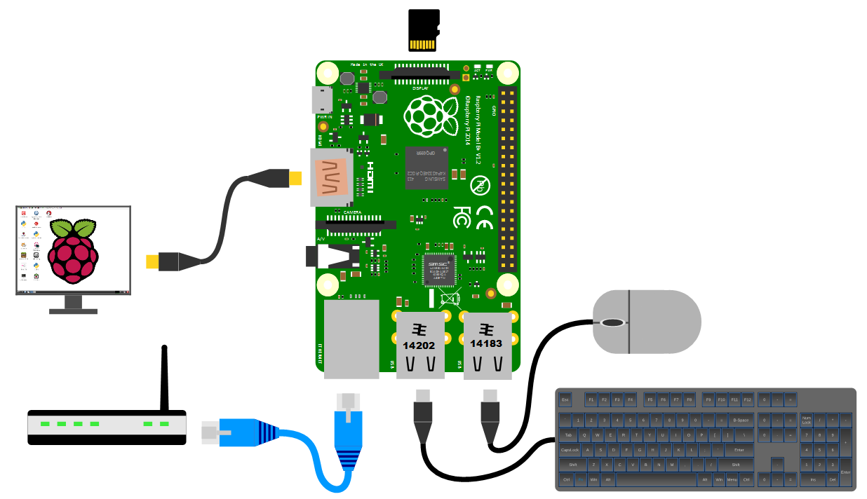
What will we need?
Well, you could just read the book and learn a bit. By itself that’s not a bad thing, but trust me when I say that actually experimenting with computers is fun and rewarding.
The list below is flexible in most cases and will depend on how you want to measure the values.
- A Raspberry Pi (I’m using a Raspberry Pi Model 3 B+ and a model 4)
- Probably a case for the Pi
- A MicroSD card
- A power supply for the Pi
- A keyboard and monitor that you can plug into the Pi (there are a few options here, read on for details)
- A remote computer (like your normal desktop PC that you can use to talk to connect to the Pi). This isn’t strictly necessary, but it makes the experience way cooler.
- An Internet connection for getting and updating the software.
As we work through the book we will be covering off the different aspects required and you should get a good overview of what your options are in different circumstances.
Why on earth did I write this rambling tome?
That’s a really good question. Writing the previous books in this series was an enjoyable process, so I thought that I’d carry on and continue to adapt the book for subsequent projects. This is book five (?, I lose track) in this series, so I suppose it’s a ‘thing’. Will this continue? Who knows, stay tuned…
Included is a bunch of information from my books on the Raspberry Pi and Linux. I hope you find it useful.
Where can you get more information?
The Raspberry Pi as a concept has provided an extensible and practical framework for introducing people to the wonders of computing in the real world. At the same time there has been a boom of information available for people to use them. The following is a far from exhaustive list of sources, but from my own experience it represents a useful subset of knowledge.
The History of the Raspberry Pi
The story of the Raspberry Pi starts in 2006 at the University of Cambridge’s Computer Laboratory. Eben Upton, Rob Mullins, Jack Lang and Alan Mycroft became concerned at the decline in the volume and skills of students applying to study Computer Science. Typical student applicants did not have a history of hobby programming and tinkering with hardware. Instead they were starting with some web design experience, but little else.
They established that the way that children were interacting with computers had changed. There was more of a focus on working with Word and Excel and building web pages. Games consoles were replacing the traditional hobbyist computer platforms. The era when the Amiga, Apple II, ZX Spectrum and the ‘build your own’ approach was gone. In 2006, Eben and the team began to design and prototype a platform that was cheap, simple and booted into a programming environment. Most of all, the aim was to inspire the next generation of computer enthusiasts to recover the joy of experimenting with computers.
Between 2006 and 2008, they developed prototypes based on the Atmel ATmega644 microcontroller. By 2008, processors designed for mobile devices were becoming affordable and powerful. This allowed the boards to support an graphical environment. They believed this would make the board more attractive for children looking for a programming-oriented device.
Eben, Rob, Jack and Alan, then teamed up with Pete Lomas, and David Braben to form the Raspberry Pi Foundation. The Foundation’s goal was to offer two versions of the board, priced at US$25 and US$35.
50 alpha boards were manufactured in August 2011. These were identical in function to what would become the model B. Assembly of twenty-five model B Beta boards occurred in December 2011. These used the same component layout as the eventual production boards.
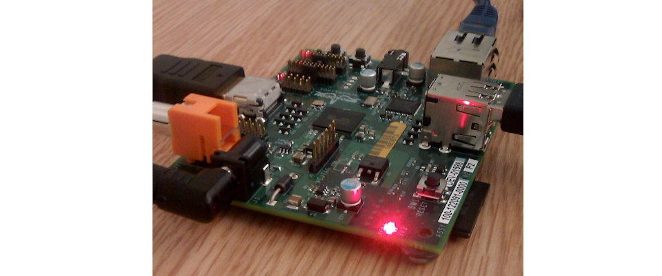
Interest in the project increased. They were demonstrated booting Linux, playing a 1080p movie trailer and running benchmarking programs. During the first week of 2012, the first 10 boards were put up for auction on eBay. One was bought anonymously and donated to the museum at The Centre for Computing History in Suffolk, England. While the ten boards together raised over 16,000 Pounds (about $25,000 USD) the last to be auctioned (serial number No. 01) raised 3,500 Pounds by itself.
The Raspberry Pi Model B entered mass production with licensed manufacturing deals through element 14/Premier Farnell and RS Electronics. They started accepting orders for the model B on the 29th of February 2012. It was quickly apparent that they had identified a need in the marketplace. Servers struggled to cope with the load placed by watchers repeatedly refreshing their browsers. The official Raspberry Pi Twitter account reported that Premier Farnell sold out within few minutes of the initial launch. RS Components took over 100,000 pre orders on the first day of sales.

Within two years they had sold over two million units.
The lower cost model A went on sale for $25 on 4 February 2013. By that stage the Raspberry Pi was already a hit. Manufacturing of the model B hit 4000 units per day and the amount of on-board ram increased to 512MB.
The official Raspberry Pi blog reported that the three millionth Pi shipped in early May 2014. In July of that year they announced the Raspberry Pi Model B+, “the final evolution of the original Raspberry Pi. For the same price as the original Raspberry Pi model B, but incorporating numerous small improvements”. In November of the same year the even lower cost (US$20) A+ was announced. Like the A, it would have no Ethernet port, and just one USB port. But, like the B+, it would have lower power requirements, a micro-SD-card slot and 40-pin HAT compatible GPIO.
On 2 February 2015 the official Raspberry Pi blog announced that the Raspberry Pi 2 was available. It had the same form factor and connector layout as the Model B+. It had a 900 MHz quad-core ARMv7 Cortex-A7 CPU, twice the memory (for a total of 1 GB) and complete compatibility with the original generation of Raspberry Pis.
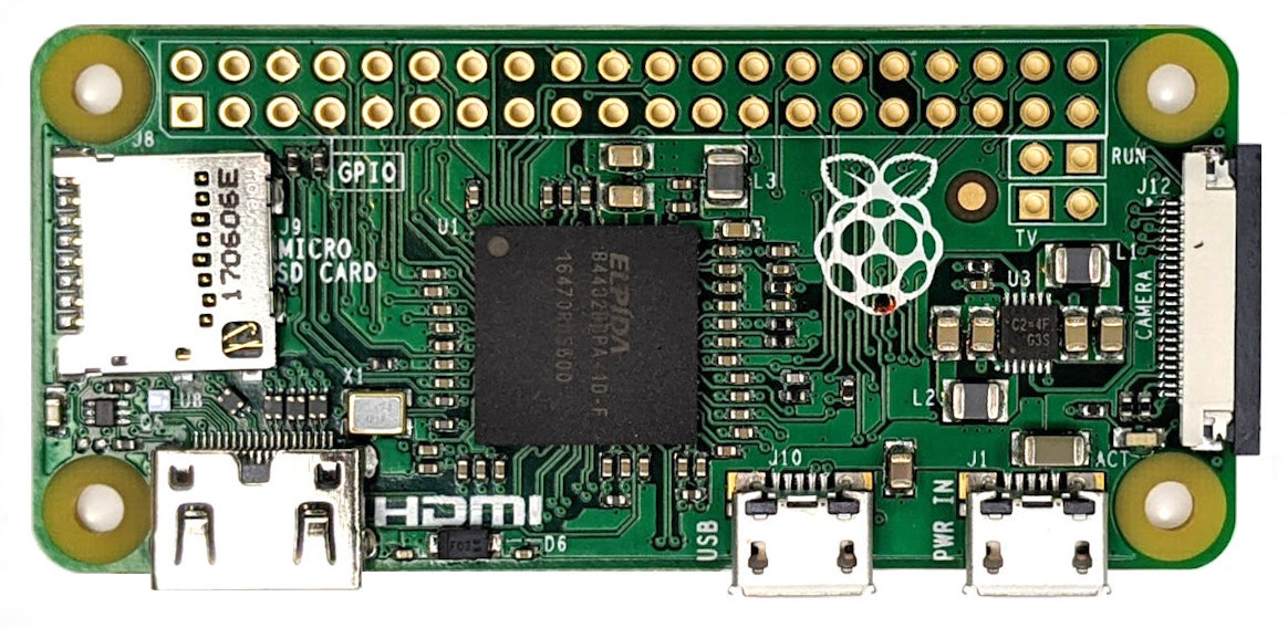
Following a meeting with Eric Schmidt (of Google fame) in 2013, Eben embarked on the design of a new form factor for the Pi. On the 26th of November 2015 the Pi Zero was released.
The Pi Zero is a significantly smaller version of a Pi with similar functionality but with a retail cost of $5. On release it sold out (20,000 units) World wide in 24 hours and a free copy was affixed to the cover of the MagPi magazine.
The Raspberry Pi 3 was released in February 2016. The most notable change being the inclusion of on-board WiFi and Bluetooth.
In February 2017 the Raspberry Pi Zero W was announced. This device had the same small form factor of the Pi Zero, but included the WiFi and Bluetooth functionality of the Raspberry Pi 3.
On Pi day (the 14th of March (Get it? 3-14?)) in 2018 the Raspberry Pi 3+ was announced. It included dual band WiFi, upgraded Bluetooth, Gigabit Ethernet and support for a future PoE card. The Ethernet speed was actually 300Mpbs since it still needs to operate on a USB2 bus. By this stage there had been over 9 million Raspberry Pi 3’s sold and 19 million Pi’s in total.
On the 24th of June 2019, the Raspberry Pi 4 was released.
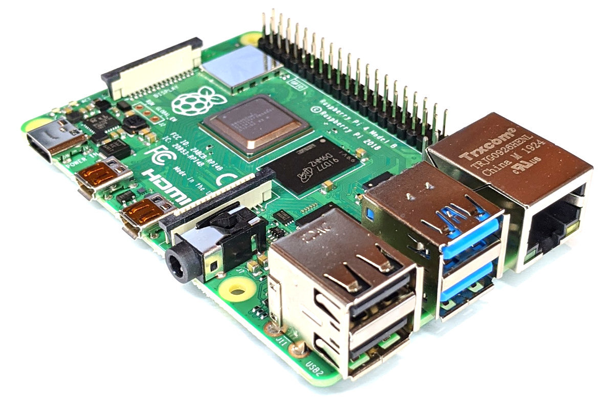
This realised a true Gigabit Ethernet port and a combination of USB 2 and 3 ports. There was also a change in layout of the board with some ports being moved and it also included dual micro HDMI connectors. As well as this, the RPi 4 is available with a wide range of on-board RAM options. Power was now supplied via a USB C port.
A new Raspberry Pi Zero W 2 was released in October 2021. This included a system in a package designed by Raspberry Pi and is capable of using a 64 bit operating system.
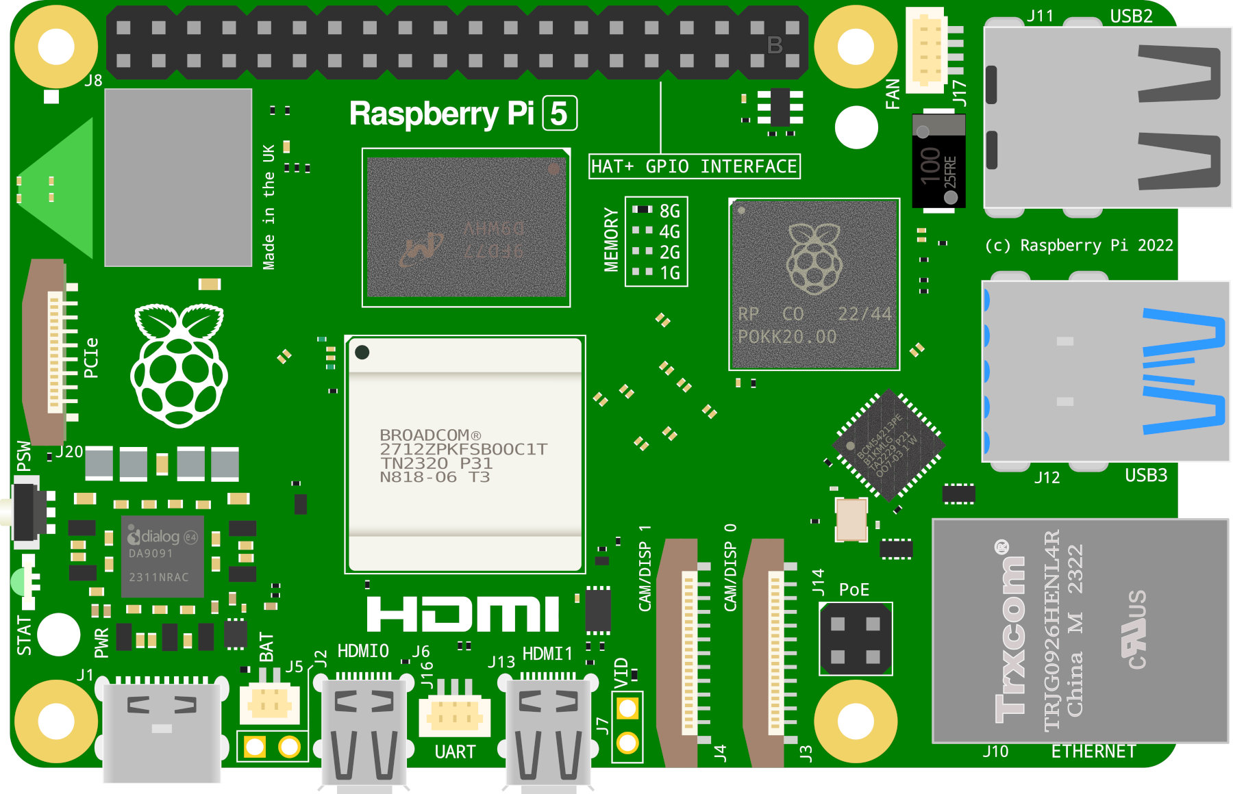
The Raspberry Pi 5 was announced on the 28th of September 2023. It features a custom input / output controller designed by Raspberry Pi and includes a clock speed of 2.4GHz for the 64-bit Cortex-A76 CPU. The dual USB 3.0 ports can now transfer up to 5 Gbps and we can connect two independent 4K 60Hz displays via the micro HDMI ports. There is now an on-board real-time clock and <gasp> a power button!
As of the 28th of February 2022 there had been over 46 million Raspberry Pis (combined) sold.
It would be easy to consider the measurement of the success of the Raspberry Pi in the number of computer boards sold. Yet, this would most likely not be the opinion of those visionaries who began the journey to develop the boards. Their stated aim was to re-invigorate the desire of young people to experiment with computers and to have fun doing it. We can thus measure their success by the many projects, blogs and updated school curriculum’s that their efforts have produced.
Raspberry Pi Versions
In the words of the totally awesome Raspberry Pi foundation;
The Raspberry Pi is a low cost, credit-card sized computer that plugs into a computer monitor or TV, and uses a standard keyboard and mouse. It’s capable of doing everything you’d expect a desktop computer to do, from browsing the internet and playing high-definition video, to making spreadsheets, word-processing, playing games and learning how to program in languages like Scratch and Python.
There are (at time of writing) fourteen different models on the market. The A, B, A+, B+, ‘model B 2’, ‘model B 3’, ‘model B 3+’, ‘model B 4’, ‘5’ (which I’m just going to call the B2, B3, B3+, 4 and 5 respectively), ‘model A+’, ‘model A+ 3’ , the Zero, Zero W and Zero 2 W. A lot of projects will typically use either the the B2, B3, B3+, 4 or the 5 for no reason other than they offer a good range of USB ports (4), 1 - 8 GB of RAM, an HMDI video connection (or two) and an Ethernet connection. For all intents and purposes either the B2, B3, B3+, 4 or 5 can be used interchangeably for the projects depending on connectivity requirements as the B3, B3+, 4 and 5 have WiFi and Bluetooth built in. For size limited situations or where lower power is an advantage, the Zero, Zero W or Zero 2 W is useful, although there is a need to cope with reduced connectivity options (a single micro USB connection) although the Zero W and Zero 2W have WiFi and Bluetooth built in. Always aim to use the latest version of the Raspberry Pi OS operating system (or at least one released on or after the 14th of March 2018). For best results browse the ‘Downloads’ page of raspberrypi.com.
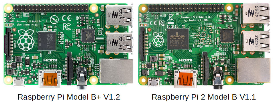
Raspberry Pi B+, B2, B3 and B3+
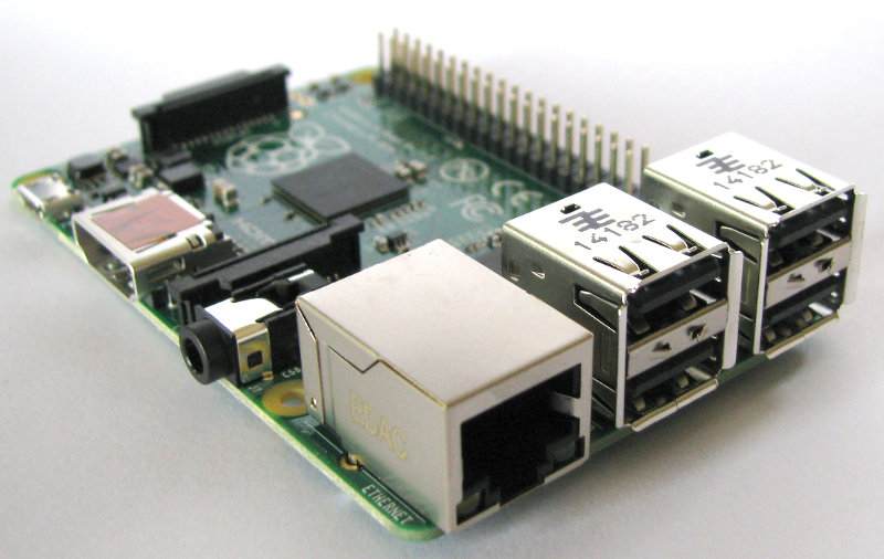
The model B+, B2, B3 and B3+ all share the same form factor and have been a consistent standard for the layout of connectors since the release of the B+ in July 2014. They measure 85 x 56 x 17mm, weighs 45g and are powered by Broadcom chipsets of varying speeds, numbers of cores and architectures.
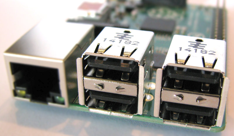
USB Ports
They include 4 x USB Ports (with a maximum output of 1.2A)
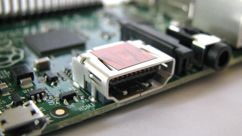
Video Out
Integrated Videocore 4 graphics GPU capable of playing full 1080p HD video via a HDMI video output connector. HDMI standards rev 1.3 & 1.4 are supported with 14 HDMI resolutions from 640×350 to 1920×1200 plus various PAL and NTSC standards.
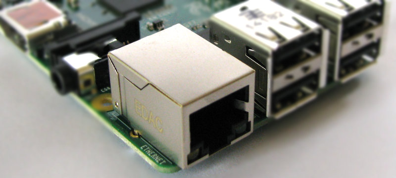
Ethernet Network Connection
There is an integrated Ethernet Port for network access. On the B2 and B3 the connection speed is fast ethernet (10/100 bps). The B3+ introduced a 300bps connection speed.
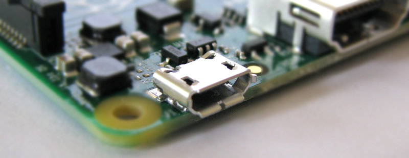
USB Power Input Jack
The boards include a 5V 2A Micro USB Power Input Jack.
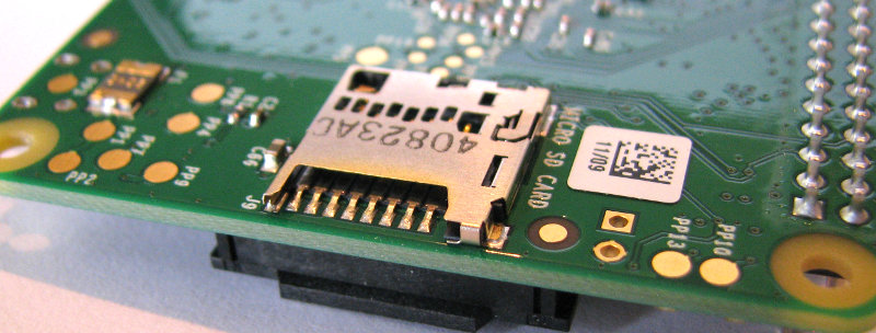
MicroSD Flash Memory Card Slot
There is a microSD card socket on the ‘underside ‘of the board. On the Model B2 this is a ‘push-push’ socket. On the B3 and later this is a simple friction fit.
Stereo and Composite Video Output
The B+, B2, B3 and B3+ includes a 4-pole (TRRS) type connector that can provide stereo sound if you plug in a standard headphone jack and composite video output with stereo audio if you use a TRRS adapter.

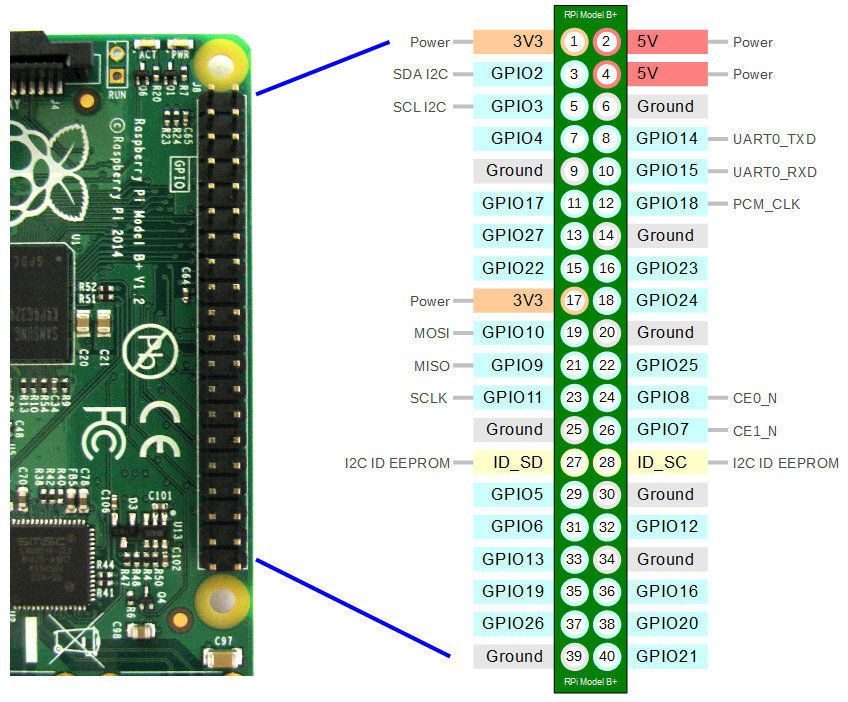
40 Pin Header
The Raspberry Pi B+, B2, B3 and B3+ include a 40-pin, 2.54mm header expansion slot (Which allows for peripheral connection and expansion boards).
Raspberry Pi 4
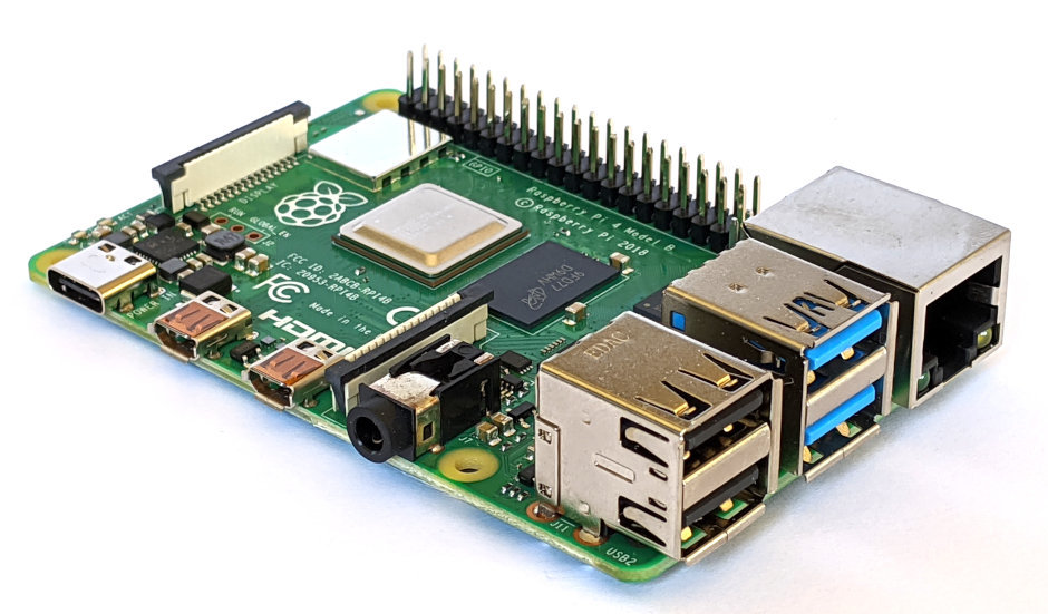
The introduction of the Raspberry Pi 4 saw the footprint of the main board used remain the same, but some of the ports have been re-arranged or changed. This means that cases for the RPi 4 will not be suitable for the B+, B2, B3 or B3+.
Pi 4 USB ports and Ethernet Ports
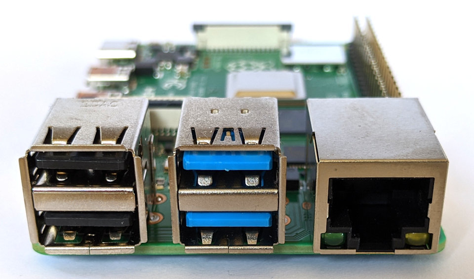
The Pi 4 includes 2 x USB 2 ports and 2 x USB 3 ports. The on-board network now supports true Gigabit speed. The location of the USB and Network ports have been reversed compared with those on the B+, B2, B3 and B3+.
Pi 4 USB C Power Input
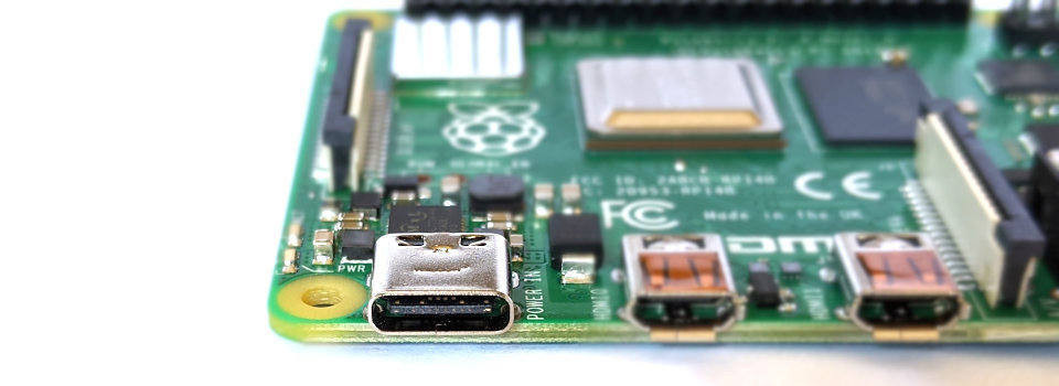
Power is now applied to the board via a USB C connector which is in the same location as the Micro USB power input jack on the B+, B2, B3 and B3+.
Pi 4 Dual Video Out
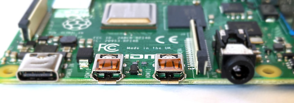
Video output is now provided via an integrated Videocore VI graphics GPU capable of displaying full 4K video via a 2 x micro-HDMI video output connectors. HDMI standard rev 2.0 is supported.
Raspberry Pi Peripherals
To make a start using the Raspberry Pi we will need to have some additional hardware to allow us to configure it.
SD Card
Traditionally the Raspberry Pi needs to store the Operating System and working files on a MicroSD card (actually a MicroSD card all models except the older A or B models which use a full size SD card). There is the ability to boot from a mass storage device or the network, but it is slightly ‘tricky’, so we won’t cover it.

The MicroSD card receptacle is on the rear of the board and on the Model B2 it is a ‘push-push’ type which means that you push the card in to insert it and then to remove it, give it a small push and it will spring out.
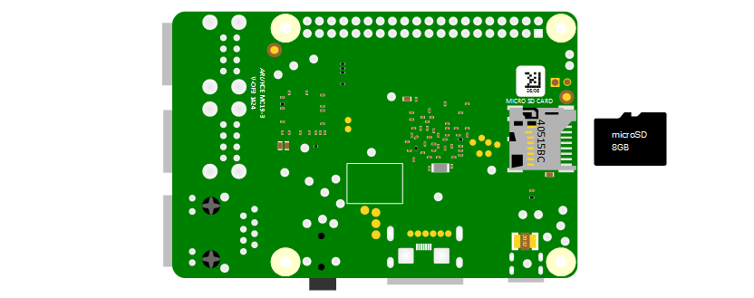
This is the equivalent of a hard drive for a regular computer, but we’re going for a minimal effect. We will want to use a minimum of an 8GB card (smaller is possible, but 8 is the realistic minimum). Also try to select a higher speed card if possible (class 10 or similar) as this will speed things up a bit.
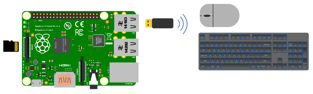
Keyboard / Mouse
While we will be making the effort to access our system via a remote computer, we will need a keyboard and a mouse for the initial set-up. Because the B+, B2, B3, B3+ and 4 models of the Pi have 4 x USB ports, there is plenty of space for us to connect wired USB devices.
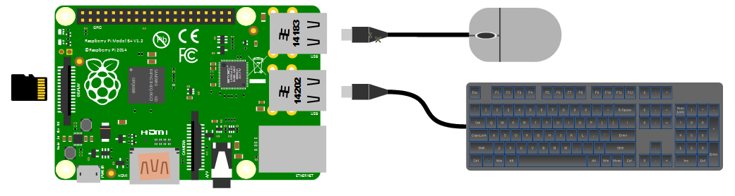
An external wireless combination would most likely be recognised without any problem and would only take up a single USB port, but if we build towards a remote capacity for using the Pi (using it headless, without a keyboard / mouse / display), the nicety of a wireless connection is not strictly required.
Video
The Raspberry Pi comes with an HDMI port ready to go which means that any monitor or TV with an HDMI connection should be able to connect easily.
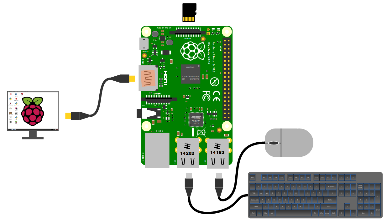
Because this is kind of a hobby thing you might want to consider utilising an older computer monitor with a DVI or 15 pin ‘D’ connector. If you want to go this way you will need an adapter to convert the connection.

Likewise, if you are using a Pi 4 or 5, the standard connectors on the board are micro HDMI and you may therefore require an adaptor.
Network
The B+, B2, B3, B3+, 4 and 5 models of the Raspberry Pi have a standard RJ45 network connector on the board ready to go. In a domestic installation this is most likely easiest to connect into a home ADSL modem or router.
This ‘hard-wired’ connection is great for getting started, but we will work through using a wireless solution later in the book.
Power supply
The Pi can be powered up in a few ways. The simplest is to use the micro USB port to connect from a standard USB charging cable for models B+, B2, B3 and B3+. You probably have a few around the house already for phones or tablets. If you are using a Pi 4 or 5 you will need a USB C power supply or an adaptor to convert between USB A and C.
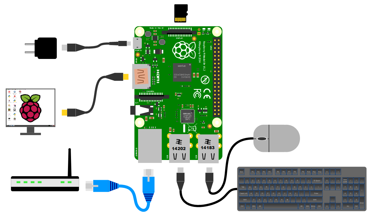
However, it’s worth thinking about the application that we use our Pi for. Depending on how much we ask of the unit, we might want to pay attention to the amount of current that our power supply can deliver. The A+, B+ and Zero models will function adequately with a 700mA supply, but the B2, B3, B3+ and 4 models will draw more current and if we want to use multiple wireless devices or supplying sensors that demand increased power, we will need to consider a supply that is capable of an output up to 2.5A. If you are thinking of including some power hungry peripherals to the Raspberry Pi 5 (because you can) you could consider a supply that could feed up to 5A.
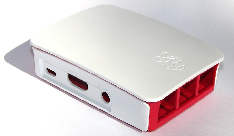
Cases
We should get ourselves a simple case to keep the Pi reasonably secure. There are a wide range of options to select from. These range from cheap but effective to more costly than the Pi itself (not hard) and looking fancy. The most important thing to consider here is to make sure you get a case appropriate to the model of Pi that you are using. Be aware that while the B+, B2, B3 and B3+ Pis share the same dimensions as the Model 4, there are differences in the port layout that means that the cases are not interchangeable
You could use a simple plastic case that can be brought for a few dollars;

For a very practical design and a warm glow from knowing that you’re supporting a worthy cause, you could go no further than the official Raspberry Pi case that includes removable side-plates and loads of different types of access. All for the paltry sum of about $9.
Operating Systems
An operating system is software that manages computer hardware and software resources for computer applications. For example Microsoft Windows could be the operating system that will allow the browser application Firefox to run on our desktop computer.
Variations on the Linux operating system are the most popular on our Raspberry Pi. Often they are designed to work in different ways depending on the function of the computer.
Linux is a computer operating system that can be distributed as free and open-source software. The defining component of Linux is the Linux kernel which was first released on 5 October 1991 by Linus Torvalds.
Linux was originally developed as a free operating system for Intel x86-based personal computers. It has since been made available to a wide range of computer hardware platforms and is one of the most popular operating systems on servers, mainframe computers and supercomputers. Linux also runs on embedded systems, which are devices whose operating system is typically built into the firmware and is highly tailored to the system; this includes mobile phones, tablet computers, network routers, facility automation controls, televisions and video game consoles. Android, the most widely used operating system for tablets and smart-phones, is built on top of the Linux kernel. In our case we will be using a version of Linux that is assembled to run on the ARM CPU architecture used in the Raspberry Pi.
The development of Linux is one of the most prominent examples of free and open-source software collaboration. Typically, Linux is packaged in a form known as a Linux ‘distribution’, for both desktop and server use. Popular mainstream Linux distributions include Debian, Ubuntu and the commercial Red Hat Enterprise Linux. Linux distributions include the Linux kernel, supporting utilities and libraries and usually a large amount of application software to carry out the distribution’s intended use.
A distribution intended to run as a server may omit all graphical desktop environments from the standard install, and instead include other software to set up and operate a solution ‘stack’ such as LAMP (Linux, Apache, MySQL and PHP). Because Linux is freely re-distributable, anyone may create a distribution for any intended use.
Welcome to Raspberry Pi OS
The Raspberry Pi OS Linux distribution is based on Debian Linux. This is the official operating system for the Raspberry Pi.
Raspberry Pi OS and Raspbian
Up until the end of May 2020 the official operating system was called ‘Raspbian’ and there will be many references to Raspbian in online and print media. With the advent of an evolution to a 64 bit architecture, the maintainers of the Raspbian code (which is 32 bit) didn’t want to have the confusion of the new 64 bit version being called Raspbian when it didn’t actually contain any of their code. So the Raspberry Pi Foundation took the opportunity to opt for a name change to simplify future operating system releases by changing the name of the official Raspberry Pi operating system to ‘Raspberry Pi OS’. The 32 bit version of Raspberry Pi OS will no doubt continue to draw from the Raspbian project, but the 64 bit version will be all new code.
Operating System Evolution
At the time of writing there have been six different operating system releases published based on the Debian Linux distribution. Those six releases are called ‘Wheezy’, ‘Jessie’, ‘Stretch’, ‘Buster’, ‘Bullseye’ and ‘Bookworm’. Debian is a widely used Linux distribution that allows Raspberry Pi OS users to leverage a huge quantity of community based experience in using and configuring software. The Wheezy edition is the earliest and was the stock edition from the inception of the Raspberry Pi till the end of 2015. From that point there were new distributions releases roughly every two years with the latest ‘Bookworm’ being released at the end of 2023. A great deal of effort goes into maintaining the ability for new Operating Systems to support the older Raspberry Pi boards. This means that you can download and install the most recent 32 bit version and it will still work on a Pi 1. However, older boards which don’t support a 64 bit architecture will not be able to run the newer 64 bit Operating Systems.
Downloading
The best place to source the latest version of the Raspberry Pi OS is to go to the raspberrypi.com page; https://www.raspberrypi.com/software/operating-systems/. We will download the ‘Lite’ version (which doesn’t use a desktop GUI). If you’ve never used a command line environment, then good news! You’re about to enter the World of ‘real’ computer users :-).
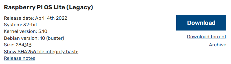
You can download via bit torrent or directly as a zip file, but whatever the method you should eventually be left with an ‘img’ file for Raspberry Pi OS.
To ensure that the projects we work on can be used with versions of the Pi from the B+ onwards we need to make sure that the version of Raspberry Pi OS we use is from 2015-01-13 or later. Earlier downloads will not support the more modern CPU of later models. To support the newer CPU of the B3+ and later (and all the previous CPUs) we will need a version of Raspberry Pi OS from 2018-03-13 or later.
We should always try to download our image files from the authoritative source!
Writing the Operating System image to the SD Card
Once we have an image file we need to get it onto our SD card.
We will work through an example using Windows 7 but the process should be very similar for other operating systems as we will be using the excellent software Raspberry Pi Imager which is available for Windows, Linux and macOS.
Download and install Raspberry Pi Imager and start it up.
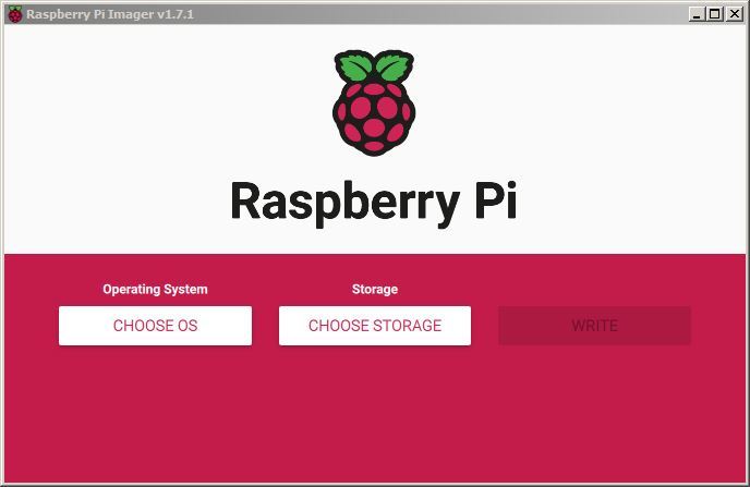
Select the ‘CHOOSE OS’ button.
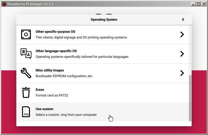
Scroll to the ‘Use custom’ option. This will allow us to have some finer degree of control over which OS we are installing.
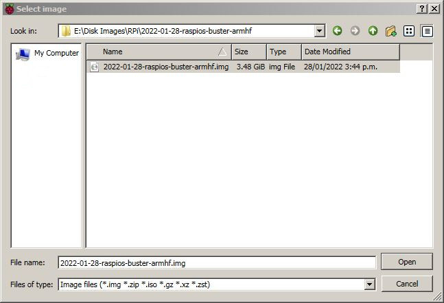
Navigate to the location of the image file that we downloaded earlier. select that and press the ‘Open’ button.
You will need an SD card reader capable of accepting your MicroSD card (you may require an adapter or have a reader built into your desktop or laptop).
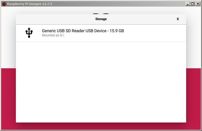
Now select the ‘CHOOSE STORAGE’ button and we will be presented with the SD card that
Assuming that your SD card is in the reader you should see Raspberry Pi Imager automatically select it for writing (Raspberry Pi Imager is very good at presenting options for installing that are only SD cards).
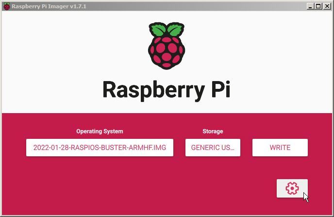
Before we write our SD card we will configure some of it’s initial settings (this is a super useful step that will save us time and effort later).
To do this click on the gear icon.
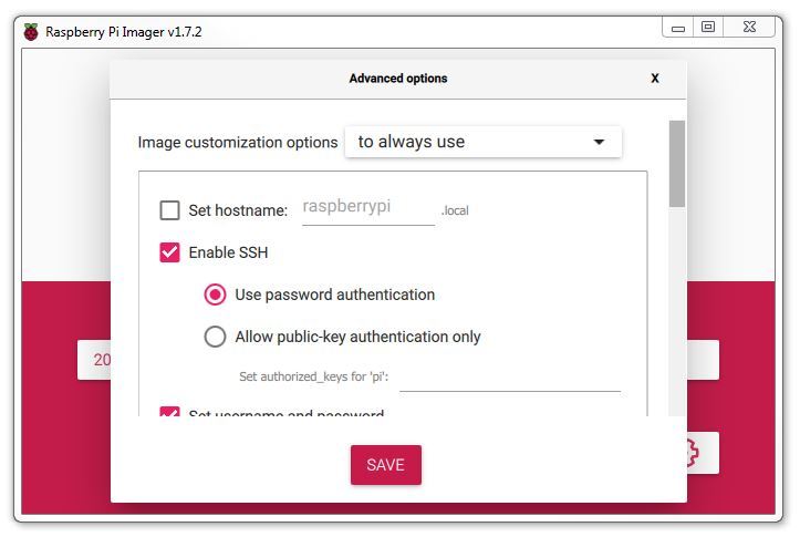
Presuming that we will want to make these options the same for future use, select the Image customisation options to ‘to always, use’
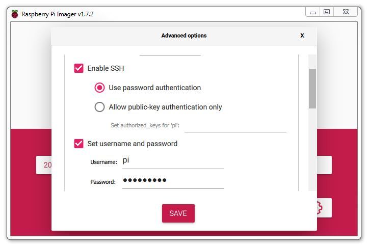
We will enable SSH so that we can remotely access the Pi and set a suitable password. Here I am setting it to the default username ‘Pi’ with the default password ‘raspberry’. You should definitely use your own username and password.
One of the awesome things when learning to use a Raspberry Pi comes when you begin to access it remotely from another computer. This is a bit of an ‘Ah Ha!’ moment for some people as they begin to appreciate just how networks and the Internet is built. We are going to enable and use remote access via what is called ‘SSH’ (this is shorthand for Secure SHell). We’ll start using it later in the book, but for now we can take the opportunity to enable it for later use.
SSH used to be enabled by default, but doing so presents a potential security concern, so it has been disabled by default as of the end of 2016. In our case it’s a feature that we want to use.
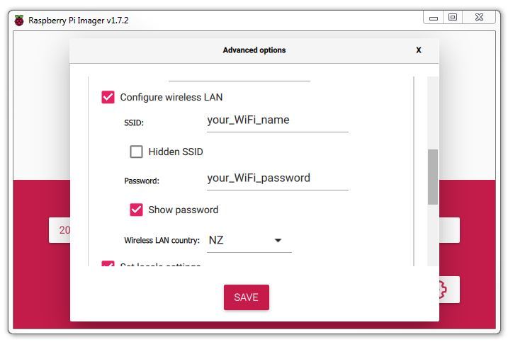
If your Pi has WiFi, you can select to configure the wireless LAN and enter it’s password. Likewise you will want to select the Wireless LAN Country for the country that you are in.
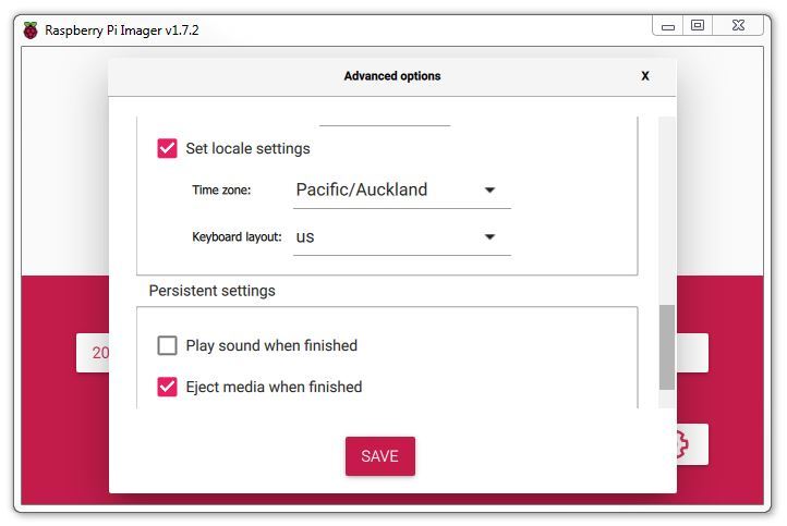
Lastly we should set our locale setting to our location and depending on your keyboard type, select the appropriate one.
Once we are happy with our settings. click on ‘SAVE’.
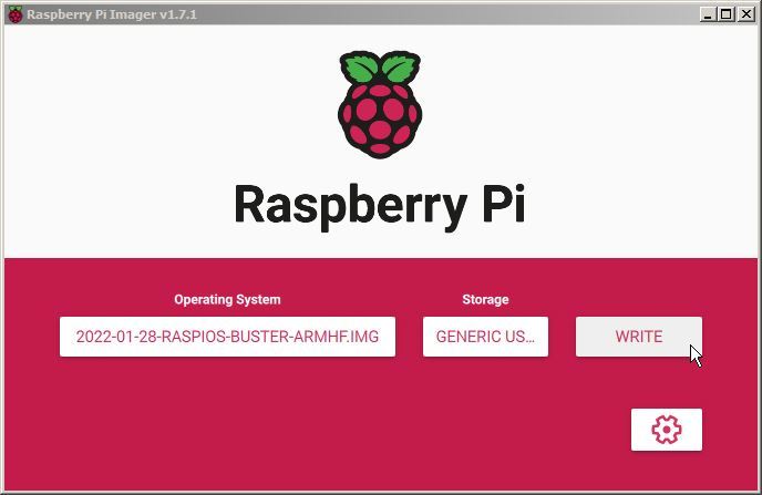
With everything ready. Click on the ‘WRITE’ button
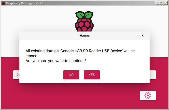
A friendly warning will let us know that if we proceed, the SD card will be erased. Press ‘YES’ if you are sure that you want to continue.
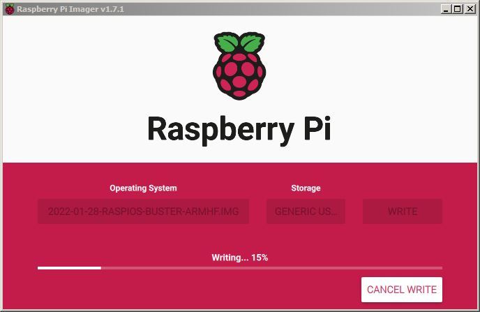
The writing process will start and progress. The time taken can vary a little, but it should only take about 3-4 minutes with a class 10 SD card.
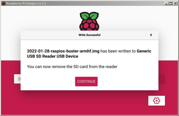
Once done, we should be told that the process has completed successfully and that we can remove our SD card.
Powering On
Insert the card into the slot on the Raspberry Pi and turn on the power.
You will see a range of information scrolling up the screen before eventually being presented with a login prompt.
The Command Line interface
Because we have installed the ‘Lite’ version of Raspberry Pi OS, when we first boot up, the process should automatically re-size the root file system to make full use of the space available on your SD card. If this isn’t the case, the facility to do it can be accessed from the Raspberry Pi configuration tool (raspi-config) that we will look at in a moment.
Once the reboot is complete (if it occurs) you will be presented with the console prompt to log on;
The default username and password (that we set earlier, buy yours may be different) is:
Username: pi
Password: raspberry
Enter the username and password.
Congratulations, you have a working Raspberry Pi and are ready to start getting into the thick of things!
If you didn’t take the opportunity to set some of the advanced options as above with the Raspberry Pi Imager, you might want to do some house keeping per below.
Raspberry Pi Software Configuration Tool
The steps in this section will only be required if you did not set them with the Raspberry Pi Imager.
We will use the Raspberry Pi Software Configuration Tool to change the locale and keyboard configuration to suit us. This can be done by running the following command;
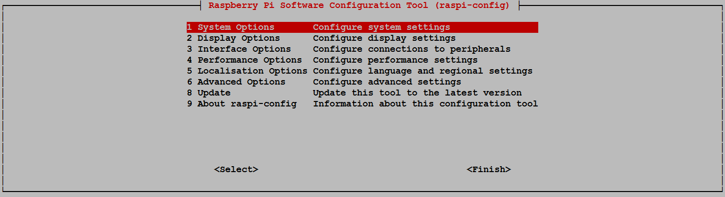
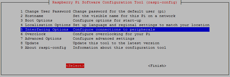
Use the up and down arrow keys to move the highlighted section to the selection you want to make then press tab to highlight the <Select> option (or <Finish> if you’ve finished).
Lets change the settings for our operating system to reflect our location for the purposes of having the correct time, language and WiFi regulations. These can all be located via selection ‘5 Localisation Options’ on the main menu.
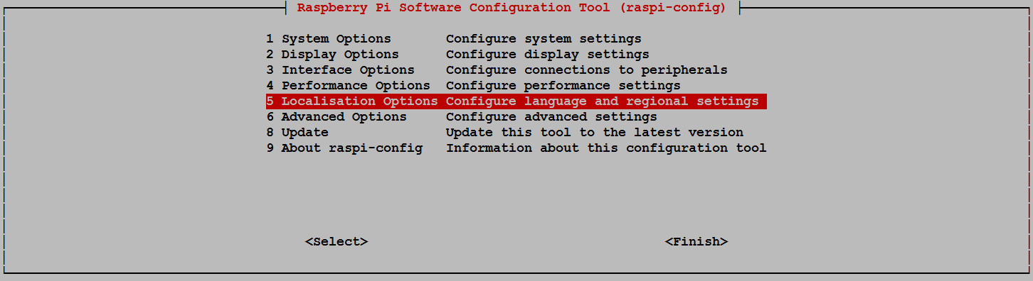
Select this and work through any changes that are required for your installation based on geography.

Once you exit out of the raspi-config menu system, if you have made a few changes, there is a possibility that you will be asked if you want to re-boot the Pi. That’s just fine. Even if you aren’t asked, it might be useful since some locales can introduce different characters on the screen.
Once the reboot is complete you will be presented with the console prompt to log on again;
Software Updates
After configuring our Pi we’ll want to make sure that we have the latest software for our system. This is a useful thing to do as it allows any additional improvements to the software we will be using to be enhanced or security of the operating system to be improved. This is probably a good time to mention that we will need to have an Internet connection available.
Type in the following line which will find the latest lists of available software;
You should see a list of text scroll up while the Pi is downloading the latest information.
Use sudo apt-key list and find the entry that is in /etc/apt/trusted.gpg.
Then we convert this entry to a .gpg file, using the last 8 numeric characters from above (90FDDD2E). The characters that you have will most likely be different!
sudo apt-key export 90FDDD2E | sudo gpg –dearmour -o /etc/apt/trusted.gpg.d/raspbian.gpg
If we have more than one warning message we can repeat the above commands for each generated by sudo apt update.
Then we want to upgrade our software to latest versions from those lists using;
The Pi should tell you the lists of packages that it has identified as suitable for an upgrade along with the amount of data that will be downloaded and the space that will be used on the system. It will then ask you to confirm that you want to go ahead. Tell it ‘Y’ and we will see another list of details as it heads off downloading software and installing it.
Power Up the Pi
To configure the Raspberry Pi for our purpose we will extend our Pi a little. This makes configuring and using the device easier and to be perfectly honest, making life hard for ourselves is so exhausting! Let’s not do that.
Static IP Address
As we mentioned earlier, enabling remote access is a really useful thing. This will allow us to configure and operate our Raspberry Pi from a separate computer. To do so we will want to assign our Raspberry Pi a static IP address.
The method by which a static address is assigned changed with the introduction of the operating system ‘bookworm’ (around the end of 2023). The older method used dhcpcd and the newer method uses nmcli. For the sake of completeness I will include both methods here.
An Internet Protocol address (IP address) is a numerical label assigned to each device (e.g., computer, printer) participating in a computer network that uses the Internet Protocol for communication.
There is a strong likelihood that our Raspberry Pi already has an IP address and it should appear a few lines above the ‘login’ prompt when you first boot up;
The My IP address... part should appear just above or around 15 lines above the login line, depending on the version of the Raspberry Pi OS we’re using. In this example the IP address 10.1.1.25 belongs to the Raspberry Pi.
This address will probably be a ‘dynamic’ IP address and could change each time the Pi is booted. For the purposes of using the Raspberry Pi with a degree of certainty when logging in to it remotely it’s easier to set a fixed IP address.
This description of setting up a static IP address makes the assumption that we have a device running on our network that is assigning IP addresses as required. This sounds complicated, but in fact it is a very common service to be running on even a small home network and most likely on an ADSL modem/router or similar. This function is run as a service called DHCP (Dynamic Host Configuration Protocol). You will need to have access to this device for the purposes of knowing what the allowable ranges are for a static IP address.
The Netmask
A common feature for home modems and routers that run DHCP devices is to allow the user to set up the range of allowable network addresses that can exist on the network. At a higher level we should be able to set a ‘netmask’ which will do the job for us. A netmask looks similar to an IP address, but it allows you to specify the range of addresses for ‘hosts’ (in our case computers) that can be connected to the network.
A very common netmask is 255.255.255.0 which means that the network in question can have any one of the combinations where the final number in the IP address varies. In other words with a netmask of 255.255.255.0, the IP addresses available for devices on the network ‘10.1.1.x’ range from 10.1.1.0 to 10.1.1.255 or in other words any one of 256 unique addresses.
CIDR Notation
An alternative to specifying a netmask in the format of ‘255.255.255.0’ is to use a system called Classless Inter-Domain Routing, or CIDR. The idea is to add a specification in the IP address itself that indicates the number of significant bits that make up the netmask.
For example, we could designate the IP address 10.1.1.17 as associated with the netmask 255.255.255.0 by using the CIDR notation of 10.1.1.17/24. This means that the first 24 bits of the IP address given are considered significant for the network routing.
Using CIDR notation allows us to do some very clever things to organise our network, but at the same time it can have the effect of confusing people by introducing a pretty complex topic when all they want to do is get their network going :-). So for the sake of this explanation we can assume that if we wanted to specify an IP address and a netmask, it could be accomplished by either specifying each separately (IP address = 10.1.1.17 and netmask = 255.255.255.0) or in CIDR format (10.1.1.17/24)
Distinguish Dynamic from Static
The other service that our DHCP server will allow is the setting of a range of addresses that can be assigned dynamically. In other words we will be able to declare that the range from 10.1.1.20 to 10.1.1.255 can be dynamically assigned which leaves 10.1.1.0 to 10.1.1.19 which can be set as static addresses.
You might also be able to reserve an IP address on your modem / router. To do this you will need to know what the MAC (or hardware address) of the Raspberry Pi is. To find the hardware address on the Raspberry Pi type;
(For more information on the ifconfig command check out the Linux commands section)
This will produce an output which will look a little like the following;
The figures b8:27:eb:b6:2e:da are the Hardware or MAC address.
Because there are a huge range of different DHCP servers being run on different home networks, I will have to leave you with those descriptions and the advice to consult your devices manual to help you find an IP address that can be assigned as a static address. Make sure that the assigned number has not already been taken by another device. In a perfect World we would hold a list of any devices which have static addresses so that our Pi’s address does not clash with any other device.
For the sake of the upcoming project we will assume that the address 10.1.1.110 is available.
Default Gateway
Before we start configuring we will need to find out what the default gateway is for our network. A default gateway is an IP address that a device (typically a router) will use when it is asked to go to an address that it doesn’t immediately recognise. This would most commonly occur when a computer on a home network wants to contact a computer on the Internet. The default gateway is therefore typically the address of the modem / router on your home network.
We can check to find out what our default gateway is from Windows by going to the command prompt (Start > Accessories > Command Prompt) and typing;
This should present a range of information including a section that looks a little like the following;
The default router gateway is therefore ‘10.1.1.1’.
For OS’s Prior to bookworm
Lets edit the dhcpcd.conf file
On the Raspberry Pi at the command line we are going to start up a text editor and edit the file that holds the configuration details for the network connections.
The file is /etc/dhcpcd.conf. That is to say it’s the dhcpcd.conf file which is in the etc directory which is in the root (/) directory.
To edit this file we are going to type in the following command;
The nano file editor will start and show the contents of the dhcpcd.conf file which should look a little like the following;
for dhcpcd.
# See dhcpcd.conf(5) for details.
# Allow users of this group to interact with dhcpcd via the control socket.
#controlgroup wheel
# Inform the DHCP server of our hostname for DDNS.
hostname
# Use the hardware address of the interface for the Client ID.
clientid
# or
# Use the same DUID + IAID as set in DHCPv6 for DHCPv4 ClientID per RFC4361.
#duid
# Persist interface configuration when dhcpcd exits.
persistent
# Rapid commit support.
# Safe to enable by default because it requires the equivalent option set
# on the server to actually work.
option rapid_commit
# A list of options to request from the DHCP server.
option domain_name_servers, domain_name, domain_search, host_name
option classless_static_routes
# Most distributions have NTP support.
option ntp_servers
# Respect the network MTU. This is applied to DHCP routes.
option interface_mtu
# A ServerID is required by RFC2131.
require dhcp_server_identifier
# Generate Stable Private IPv6 Addresses instead of hardware based ones
slaac private
# Example static IP configuration:
#interface eth0
#static ip_address=192.168.0.10/24
#static ip6_address=fd51:42f8:caae:d92e::ff/64
#static routers=192.168.0.1
#static domain_name_servers=192.168.0.1 8.8.8.8 fd51:42f8:caae:d92e::1
# It is possible to fall back to a static IP if DHCP fails:
# define static profile
#profile static_eth0
#static ip_address=192.168.1.23/24
#static routers=192.168.1.1
#static domain_name_servers=192.168.1.1
# fallback to static profile on eth0
#interface eth0
#fallback static_eth0
The file actually contains some commented out sections that provide guidance on entering the correct configuration.
We are going to add the information that tells the network interface to use eth0 at our static address that we decided on earlier (10.1.1.110) along with information on the netmask to use (in CIDR format) and the default gateway of our router. To do this we will add the following lines to the end of the information in the dhcpcd.conf file;
Here we can see the IP address and netmask (static ip_address=10.1.1.110/24), the gateway address for our router (static routers=10.1.1.1) and the address where the computer can also find DNS information (static domain_name_servers=10.1.1.1).
Once you have finished press ctrl-x to tell nano you’re finished and it will prompt you to confirm saving the file. Check your changes over and then press ‘y’ to save the file (if it’s correct). It will then prompt you for the file-name to save the file as. Press return to accept the default of the current name and you’re done!
To allow the changes to become operative we can type in;
This will reboot the Raspberry Pi and we should see the (by now familiar) scroll of text and when it finishes rebooting you should see;
Which tells us that the changes have been successful (bearing in mind that the IP address above should be the one you have chosen, not necessarily the one we have been using as an example).
For OS’s From bookworm onward
From late 2023 on (assuming that you’re using the latest available Operating System), the default command line tool for setting a static IP address changed to nmcli (nccli is the command line interface tool for the NetworkManager package.
Using this tool means that there is no editing of configuration files required.
To find the name of the connection that we are going to change we run the nmcli con show command. (this is basically shorthand for saying “Show the connections nmcli!”.
This will produce something like the following;
From our checking we know that;
-
Wired connection 1is the name of the connection that we will be setting to a static IP address -
10.1.1.110/24is the static IP address and the netmask that we want (in CIDR notation) -
10.1.1.1is our gateway -
10.1.1.1is also our the address where the computer can go to find DNS information.
Now we can run the commands that will set the Static IP address with all our desired parameters as follows;
We could have actually strung all those commands together as a single command, but for the sake of formatting in the book, the above avoids confusion with line breaks.
To save the changes and reload the network manager we run the following command;
All that remains is to reboot the Pi for the changes to take effect;
This will reboot the Raspberry Pi and we should see the (by now familiar) scroll of text and when it finishes rebooting you should see;
Which tells us that the changes have been successful (bearing in mind that the IP address above should be the one you have chosen, not necessarily the one we have been using as an example).
Remote access
To allow us to work on our Raspberry Pi from our normal desktop we can give ourselves the ability to connect to the Pi from another computer. The will mean that we don’t need to have the keyboard / mouse or video connected to the Raspberry Pi and we can physically place it somewhere else and still work on it without problem. This process is called ‘remotely accessing’ our computer .
To do this we need to install an application on our windows desktop which will act as a ‘client’ in the process and have software on our Raspberry Pi to act as the ‘server’. There are a couple of different ways that we can accomplish this task, but because we will be working at the command line (where all we do is type in our commands (like when we first log into the Pi)) we will use what’s called SSH access in a ‘shell’.
Remote access via SSH
Secure SHell (SSH) is a network protocol that allows secure data communication, remote command-line login, remote command execution, and other secure network services between two networked computers. It connects, via a secure channel over an insecure network, a server and a client running SSH server and SSH client programs, respectively (there’s the client-server model again).
In our case the SSH program on the server is running sshd and on the Windows machine we will use a program called ‘PuTTY’.
Setting up the Server (Raspberry Pi)
SSH is already installed and operating but to check that it is there and working type the following from the command line;
The Pi should respond with the message that the program sshd is active (running).
(/lib/systemd/system/ssh.service; enabled)
Active: active (running) since Tue 2017-04-25 03:30:16 UTC; 1h 28min ago
Main PID: 2135 (sshd)
CGroup: /system.slice/ssh.service
└─2135 /usr/sbin/sshd -D
If it isn’t, run the following command;
Use the up and down arrow keys to move the highlighted section to the selection you want to make then press tab to highlight the <Select> option (or <Finish> if you’ve finished).
To enable SSH select ‘5 Interfacing Options’ from the main menu.
From here we select ‘P2 SSH’
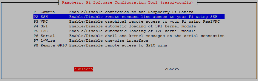
And we should be done!
Setting up the Client (Windows)
The client software we will use is called ‘Putty’. It is open source and available for download from here.
On the download page there are a range of options available for use. The best option for us is most likely under the ‘For Windows on Intel x86’ heading and we should just download the ‘putty.exe’ program.
Save the file somewhere logical as it is a stand-alone program that will run when you double click on it (you can make life easier by placing a short-cut on the desktop).
Once we have the file saved, run the program by double clicking on it and it will start without problem.
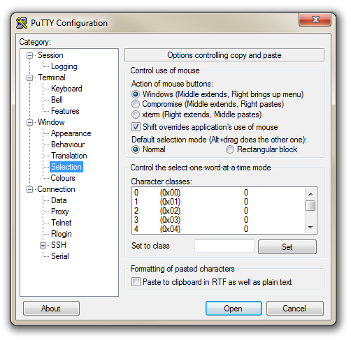
The first thing we will set-up for our connection is the way that the program recognises how the mouse works. In the ‘Window’ Category on the left of the PuTTY Configuration box, click on the ‘Selection’ option. On this page we want to change the ‘Action of mouse’ option from the default of ‘Compromise (Middle extends, Right paste)’ to ‘Windows (Middle extends, Right brings up menu)’. This keeps the standard Windows mouse actions the same when you use PuTTY.
Now select the ‘Session’ Category on the left hand menu. Here we want to enter our static IP address that we set up earlier (10.1.1.160 in the example that we have been following, but use your one) and because we would like to access this connection on a frequent basis we can enter a name for it as a saved session (In the screen-shot below it is imaginatively called ‘Raspberry Pi’). Then click on ‘Save’.
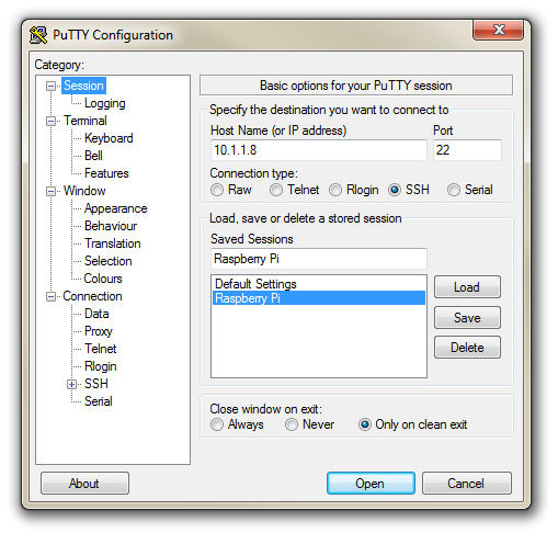
Now we can select our Raspberry Pi session (per the screen-shot above) and click on the ‘Open’ button.
The first thing you will be greeted with is a window asking if you trust the host that you’re trying to connect to.
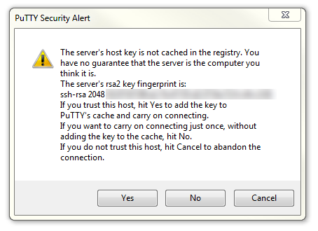
In this case it is a pretty safe bet to click on the ‘Yes’ button to confirm that we know and trust the connection.
Once this is done, a new terminal window will be shown with a prompt to login as: . Here we can enter our user name (‘pi’) and then our password (if it’s still the default, the password is ‘raspberry’).
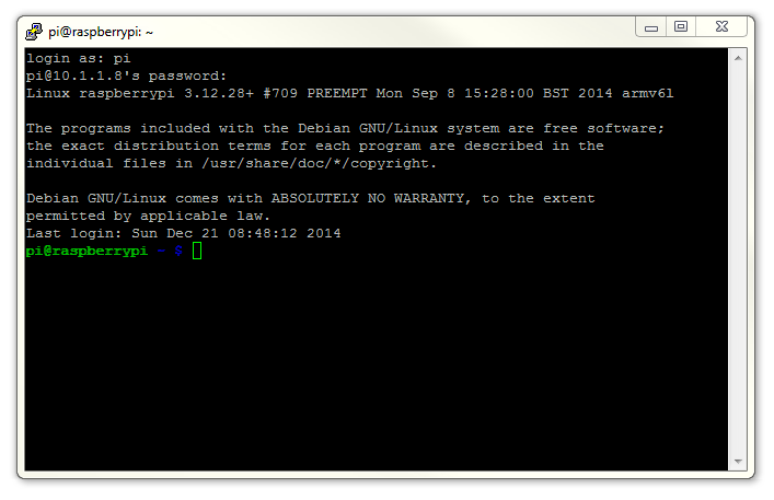
There you have it. A command line connection via SSH. Well done.
WinSCP
To make the process of transferring files from Windows easier I would recommend looking to the program WinSCP. (If you’re using Linux I will make the assumption that you know how to do the equivalent using SCP.)
This provides a very intuitive way to copy files between your desktop and the Pi.
Download and install the program. Once installed, click on the desktop icon.
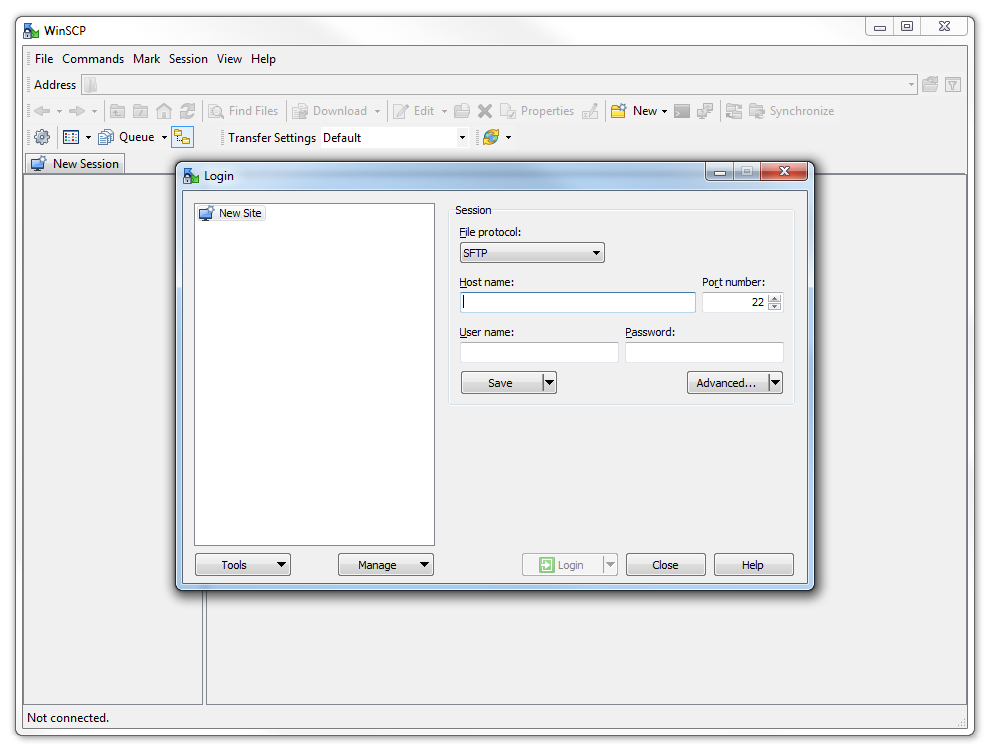
The program opens with default login page. Enter the ‘Host name’ field with the IP address of the Pi. Also put in the username and password of the Pi.
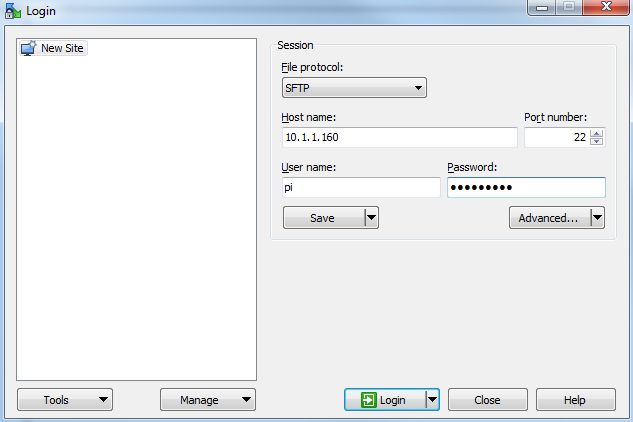
Click on ‘Save’ to save the login details for ease of future access.
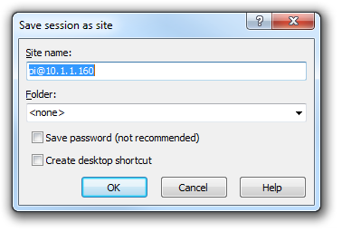
Enter the ‘Site name’ as a name of the Pi or leave it as the default, with the user and IP address. Check the ‘Save password’ for a convenient but insecure way to avoid typing in the username and password in the future. Then press OK
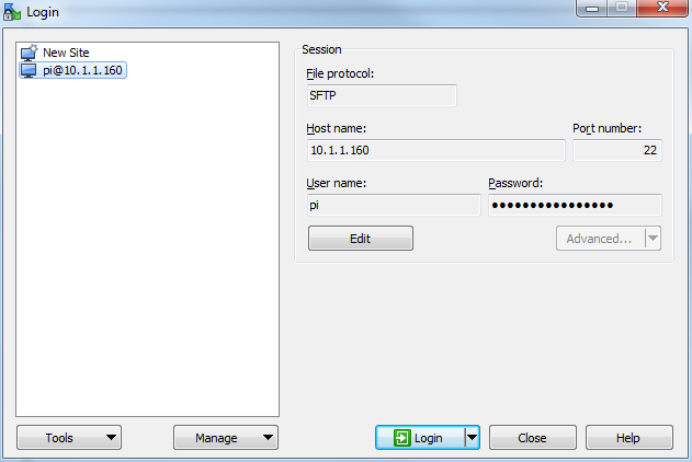
The saved login details now appear on the left hand pane. Click on ‘Login’ to log in to the Pi.
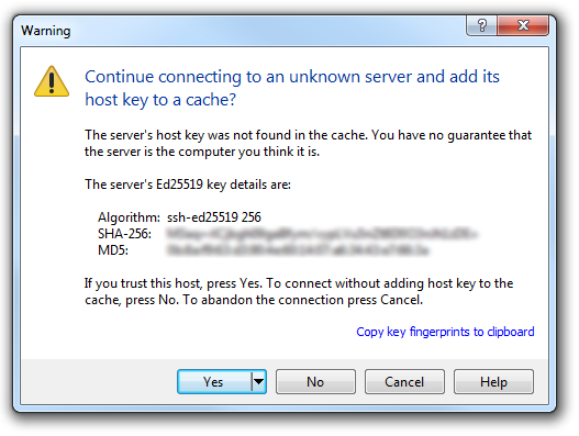
We will receive a warning about connecting to an unknown server for the first time. Assuming that we are comfortable doing this (i.e. that we know that we are connecting the Pi correctly) we can click on ‘Yes’.
There is a possibility that it might fail on its first attempt, but tell it to reconnect if it does and we should be in!
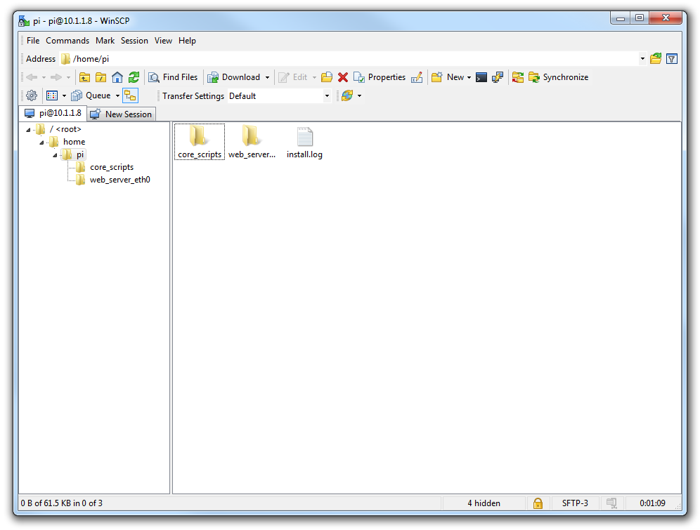
Here we can see a familiar tree structure for file management and we have the ability to copy files via dragging and dropping them into place.
Assuming that we already have PuTTY installed we should be able to click on the ‘Open Session in PuTTY’ icon and we will get access to the command line.
If this is the first time that you’ve done something like this (remotely accessing a computer) it can be a very liberating feeling. Nice job.
Setting up a WiFi Network Connection
Our set-up of the Raspberry Pi will allow us to carry out all the (computer interface) interactions via a remote connection. However, the Raspberry Pi is currently making that remote connection via a fixed network cable. It could be argued that the lower number of connections that we need to run to our machine the better. The most obvious solution to this conundrum is to enable a wireless connection.
It should be noted that enabling a wireless network will not be a requirement for everyone, and as such, I would only recommend it if you need to. If you’re using a model B3, B3+, 4, 5, Zero W or Zero 2W you have WiFi built in, otherwise you will need to purchase a USB WiFi dongle and correctly configure it.
We should also note that the configuration of your WiFi connection can be set using the Raspberry Pi Imager as mentioned earlier in the book.
Built in WiFi Enabling
We need to edit the file wpa_supplicant.conf at /etc/wpa_supplicant/wpa_supplicant.conf. This looks like the following;
Use the nano command as follows;
We need to add the ssid (the wireless network name) and the password for the WiFi network here so that the file looks as follows (using your ssid and password of course);
Make the changes operative
To allow the changes to become operative we can type in;
Once we have rebooted, we can check the status of our network interfaces by typing in;
This will display the configuration for our wired Ethernet port, our ‘Local Loopback’ (which is a fancy way of saying a network connection for the machine that you’re using, that doesn’t require an actual network (ignore it in the mean time)) and the wlan0 connection which should look a little like this;
flags=4163<UP,BROADCAST,RUNNING,MULTICAST> mtu 1500
inet 10.1.1.99 netmask 255.255.255.0 broadcast 10.1.1.255
inet6 fe80::8b9f:3e4f:dcf0:12a9 prefixlen 64 scopeid 0x20<link>
ether b8:27:eb:e3:b7:f2 txqueuelen 1000 (Ethernet)
RX packets 51 bytes 9384 (9.1 KiB)
RX errors 0 dropped 0 overruns 0 frame 0
TX packets 35 bytes 6078 (5.9 KiB)
TX errors 0 dropped 0 overruns 0 carrier 0 collisions 0
This would indicate that our wireless connection has been assigned the dynamic IP address 10.1.1.99.
We should be able to test our connection by connecting to the Pi via SSH and ‘PuTTY’ on the Windows desktop using the address 10.1.1.99.
In theory you are now the proud owner of a computer that can be operated entirely separate from all connections except power!
Make the built in WiFi IP address static
In the same way that we would edit the /etc/dhcpcd.conf file to set up a static IP address for our physical connection (eth0) we will now edit it with the command…
This time we will add the details for the wlan0 connection to the end of the file. Those details (assuming we will use the 10.1.1.17 IP address) should look like the following;
Our wireless lan (wlan0) is now designated to be a static IP address (with the details that we had previously assigned to our wired connection) and we have added the ‘ssid’ (the network name) of the network that we are going to connect to and the password for the network.
Make the changes operative
To allow the changes to become operative we can type in;
We’re done!
WiFi Via USB Dongle
Using an external USB WiFi dongle can be something of an exercise if not done right. In my own experience, I found that choosing the right wireless adapter was the key to making the job simple enough to be able to recommend it to new users. Not all WiFi adapters are well supported and if you are unfamiliar with the process of installing drivers or compiling code, then I would recommend that you opt for an adapter that is supported and will work ‘out of the box’. There is an excellent page on elinux.org which lists different adapters and their requirements. I eventually opted for the Edimax EW-7811Un which literally ‘just worked’ and I would recommend it to others for it’s ease of use and relatively low cost (approximately $15 US).

To install the wireless adapter we should start with the Pi powered off and install it into a convenient USB connection. When we turn the power on we will see the normal range of messages scroll by, but if we’re observant we will note that there are a few additional lines concerning a USB device. These lines will most likely scroll past, but once the device has finished powering up and we have logged in we can type in…
… which will show us a range of messages about drivers that are loaded to support discovered hardware.
Somewhere in that list (hopefully towards the end) will be a series of messages that describe the USB connectors and what is connected to them. In particular we could see a group that looks a little like the following;
That is our USB adapter which is plugged into USB slot 2 (which is the ‘2’ in usb 1-1.2:). The manufacturer is listed as ‘Realtek’ as this is the manufacturer of the chip-set in the adapter that Edimax uses.
Editing files
We need to edit two files. The first is the file wpa_supplicant.conf at /etc/wpa_supplicant/wpa_supplicant.conf. This looks like the following;
Use the nano command as follows;
We need to add the ssid (the wireless network name) and the password for the WiFi network here so that the file looks as follows (using your ssid and password of course);
Make the changes operative
To allow the changes to become operative we can type in;
Once we have rebooted, we can check the status of our network interfaces by typing in;
This will display the configuration for our wired Ethernet port, our ‘Local Loopback’ (which is a fancy way of saying a network connection for the machine that you’re using, that doesn’t require an actual network (ignore it in the mean time)) and the wlan1 connection which should look a little like this;
flags=4163<UP,BROADCAST,RUNNING,MULTICAST> mtu 1500
inet 10.1.1.97 netmask 255.255.255.0 broadcast 10.1.1.255
inet6 fe80::c4e4:a6e5:9788:d2c2 prefixlen 64 scopeid 0x20<link>
ether 00:ec:0b:4c:6b:99 txqueuelen 1000 (Ethernet)
RX packets 106 bytes 18616 (18.1 KiB)
RX errors 0 dropped 0 overruns 0 frame 0
TX packets 34 bytes 5681 (5.5 KiB)
TX errors 0 dropped 0 overruns 0 carrier 0 collisions 0
This would indicate that our wireless connection has been assigned the dynamic IP address 10.1.1.97.
We should be able to test our connection by connecting to the Pi via SSH and ‘PuTTY’ on the Windows desktop using the address 10.1.1.97.
Make USB WiFi IP address static
In the same way that we would edit the /etc/dhcpcd.conf file to set up a static IP address for our physical connection (eth0) we will now edit it with the command…
This time we will add the details for the wlan1 connection to the end of the file. Those details (assuming we will use the 10.1.1.110 IP address) should look like the following;
Make the changes operative
To allow the changes to become operative we can type in;
We’re done!
About Prometheus
Prometheus is an open source application used for monitoring and alerting. It records real-time metrics in a time series database built using a HTTP pull model.
It is licensed under the Apache 2 License, with source code available on GitHub.
It was was created because of the need to monitor multiple microservices that might be running in a system. It employs a modular architecture and employs modules called exporters, which allow the capture of metrics from a range of platforms, IT hardware and software. Prometheus is written with easily distributed binaries which allow it to run standalone with no external dependencies.
Prometheus’s ‘pull model’ of metrics gathering means that it will actively request information for recording. The alternative (and both have strengths) is a ‘push model’ which occurs when information is pushed to a recording service without being asked. InfluxDB is a popular piece of software that employs that model.
Prometheus collects metrics at regular intervals and stores them locally. These metrics are pulled from nodes that run ‘exporters’. An exporter can be defined as a module that extracts information and translates it into the Prometheus format.
Prometheus has an alert manager that can notify a follow on end point if something is awry and it has a visualisation component that is useful for testing. However, it is commonly used in combination with the Grafana platform which has a very powerful visualisation capability.
Prometheus data is stored as metrics, with each having a name that is used for referencing and querying. This is what makes it very good at recording time series data. To add dimensionality, each metric can be drilled down by an arbitrary number of key=value pairs (labels). Labels can include information on the data source and other application-specific information.
About Grafana
Grafana is an open-source, general purpose dashboard and visualisation tool, which runs as a web application. It supports a range of data inputs such as InfluxDB or Prometheus.
It allows you to visualize and alert on your metrics as well as allowing for the creation of dynamic & reusable dashboards.
Grafana is open source and covered by the Apache 2.0 license and its source code is available on GitHub.
Three of the primary strengths of Grafana are;
- A powerful engine for the building of dashboards that can contain a wide range of different visualisation techniques.
- The ability to display dynamic data from multiple sources in a way that allows for multi-dimensional integration.
- An alerting engine that provides the ability to attach rules to dashboard panels. These rules provide the facility to trigger alerts and notifications.
Installation
While the Raspberry Pi comes with a range of software already installed on the Raspberry Pi OS distribution (even the Lite version) we will need to download and install Prometheus and Grafana separately
If you’re sneakily starting reading from this point, make sure that you update and upgrade the Raspberry Pi OS before continuing.
Installing Prometheus
The first thing that we will want to do before installing Prometheus is to determine what the latest version is. To do this browse to the download page here - https://prometheus.io/download/. There are a number of different software packages available, but it’s important before looking at any of them that we select the correct architecture for our Raspberry Pi. As the Pi 4 (which I’m using for this install) uses a CPU based on the Arm v7 architecture, use the drop-down box to show armv7 options.
Note the name or copy the URL for the file that is presented. On the 7th of January 2024, the version that was available was 2.48.1. The full URL was something like;
https://github.com/prometheus/prometheus/releases/download/v2.48.1/prometheus-2.4\
8.1.linux-armv7.tar.gz
We can see that ‘armv7’ is even in the name. That’s a great way to confirm that we’re on the right track.
On our Pi we will start the process in the pi users home directory (/home/pi/). We will initiate the download process with the wget command as follows (the command below will break across lines, don’t just copy - paste it);
The file that is downloaded is compressed so once the download is finished we will want to expand our file. For this we use the tar command;
Let’s do some housekeeping and remove the original compressed file with the rm (remove) command;
We now have a directory called prometheus-2.48.1.linux-armv7. While that’s nice and descriptive, for the purposes of simplicity it will be easier to deal with a directory with a simpler name. We will therefore use the mv (move) command to rename the directory to just ‘prometheus’ thusly;
Believe it or not, that is as hard as the installation gets. Everything from here is configuration in one form or another. However, the first part of that involves making sure that Prometheus starts up simply at boot. We will do this by setting it up as a service so that it can be easily managed and started.
The first step in this process is to create a service file which we will call prometheus.service. We will have this in the /etc/systemd/system/ directory.
Paste the following text into the file and save and exit.
The service file can contain a wide range of configuration information and in our case there are only a few details. The most interesting being the ‘ExecStart’ details which describe where to find the prometheus executable and what options it should use when starting. In particular we should note the location of the prometheus.yml file which we will use in the future when adding things to monitor to Prometheus.
Before starting our new service we will need to reload the systemd manager configuration. This essentially takes changed configurations from our file system and makes them ready to be used. We have added a service, so systemd needs to know about it before it can start it.
Now we can start the Prometheus service. .
You shouldn’t see any indication at the terminal that things have gone well, so it’s a good idea to check Prometheus’s status as follows;
We should see a report back that indicates (amongst other things) that Prometheus is active and running.
Now we will enable it to start on boot.
To check that this is all working well we can use a browser to verify that Prometheus is serving metrics about itself by navigating to its own metrics endpoint at http://10.1.1.110:9090/metrics (or at least at the IP address of your installation).
A long list of information should be presented in the browser that will look a little like the following;
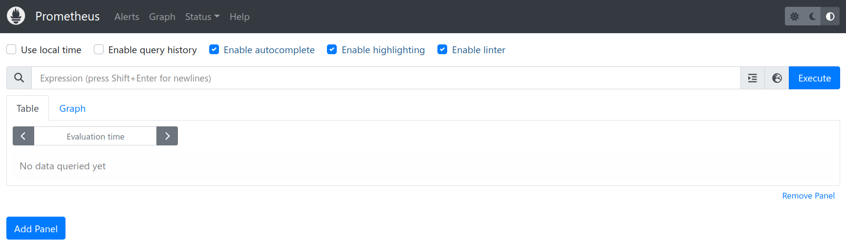
We can now go to a browser and enter the IP address of our installation with the port :9090 to confirm that Prometheus is operating. In our case that’s http://10.1.1.110:9090.
If we now go to the ‘Status’ drop down menu and select ‘Targets’ we can see the list of targets that Prometheus is currently scraping metrics from.
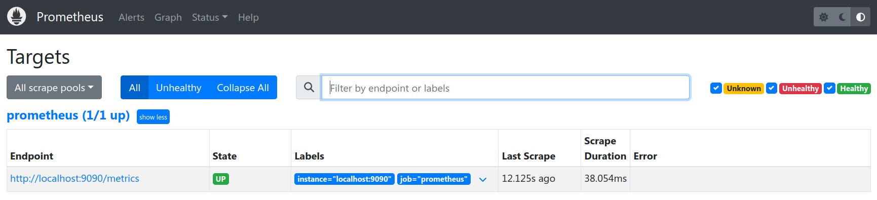
From the information above, we can see that it is already including itself as a metric monitoring point!
There’s still plenty more to do on configuring Prometheus (specifically setting up exporters), but for the mean time we will leave the process here and set up Grafana.
Installing Grafana
There are two different ways that we can go about installing Grafana. Manually, in a way very much like the one that we used for Prometheus, or via the package management service ‘apt-get’. Both methods will be described below, but I will recommend the ‘apt-get’ method as it is simpler and allows for easier updating.
Installing Grafana Manually
In much the same way that we installed Prometheus, the first thing we need to do is to find the right version of Grafana to download. To do this browse to the download page here - https://grafana.com/grafana/download?platform=arm. There are a number of different ways to install Grafana. We are going to opt for the simple method of installing a standalone binary in much the same way that we installed Prometheus.
The download page noted above goes straight to the ARM download page. We will be looking for the ‘Standalone Linux Binaries’ for ARMv7. Note the name or copy the URL for the file that is presented. On the 7th of January 20224, the version that was available was 10.2.3. The full URL was something like https://dl.grafana.com/oss/release/grafana-enterprise-10.2.3.linux-armv7.tar.gz;
On our Pi we will start the process in the pi users home directory (/home/pi/). We will initiate the download process with the wget command as follows (the command below will break across lines, don’t just copy - paste it);
The file that is downloaded is compressed so once the download is finished we will want to expand our file. For this we use the tar command;
Housekeeping time again. Remove the original compressed file with the rm (remove) command;
We now have a directory called grafana-10.2.3. While that’s nice and descriptive, for the purposes of simplicity it will be easier to deal with a directory with a simpler name. We will therefore use the mv (move) command to rename the directory to just ‘grafana’ thusly;
Again, now we need to make sure that Grafana starts up simply at boot. We will do this by setting it up as a service so that it can be easily managed and started.
The first step in this process is to create a service file which we will call grafana.service. We will have this in the /etc/systemd/system/ directory.
Paste the following text into the file and save and exit.
The service file can contain a wide range of configuration information and in our case there are only a few details. The most interesting being the ‘ExecStart’ details which describe where to find the Grafana executable.
Before starting our new service we will need to reload the systemd manager configuration again.
Now we can start the Grafana service.
You shouldn’t see any indication at the terminal that things have gone well, so it’s a good idea to check Grafana’s status as follows;
We should see a report back that indicates (amongst other things) that Grafana is active and running.
Now we will enable it to start on boot.
Installing Grafana Automatically Using ‘apt-get’
So while we call this an automatic method, there is still some manual work to set things up at the start.
First we need to add the APT key used to authenticate the packages:
If we’re using one of the more modern versions of Raspberry Pi OS we may get a warning that apt-key is deprecated. There will come a time in the future when we will need to move to trusted.gpg.d, but that will be a job for our future selves.
Now we need to add the Grafana APT repository (the command below will break across lines, don’t just copy - paste it):
With those pieces of set-up out of the way we can install Grafana;
Grafana is now installed but to make sure that it starts up when the our Pi is restarted, we need to enable and start the Grafana Systemctl service.
First enable the Grafana server;
Then start the Grafana server;
Using Grafana
At this point we have Grafana installed and configured to start on boot. Let’s start exploring!
Using a browser, connect to the Grafana server: http://10.1.1.110:3000.
The account and password are: admin/admin. Grafana will ask you to change this password.
The first configuration to be made will be to create a data source that Grafana will use to collect metrics. Of course, this will be our Prometheus instance
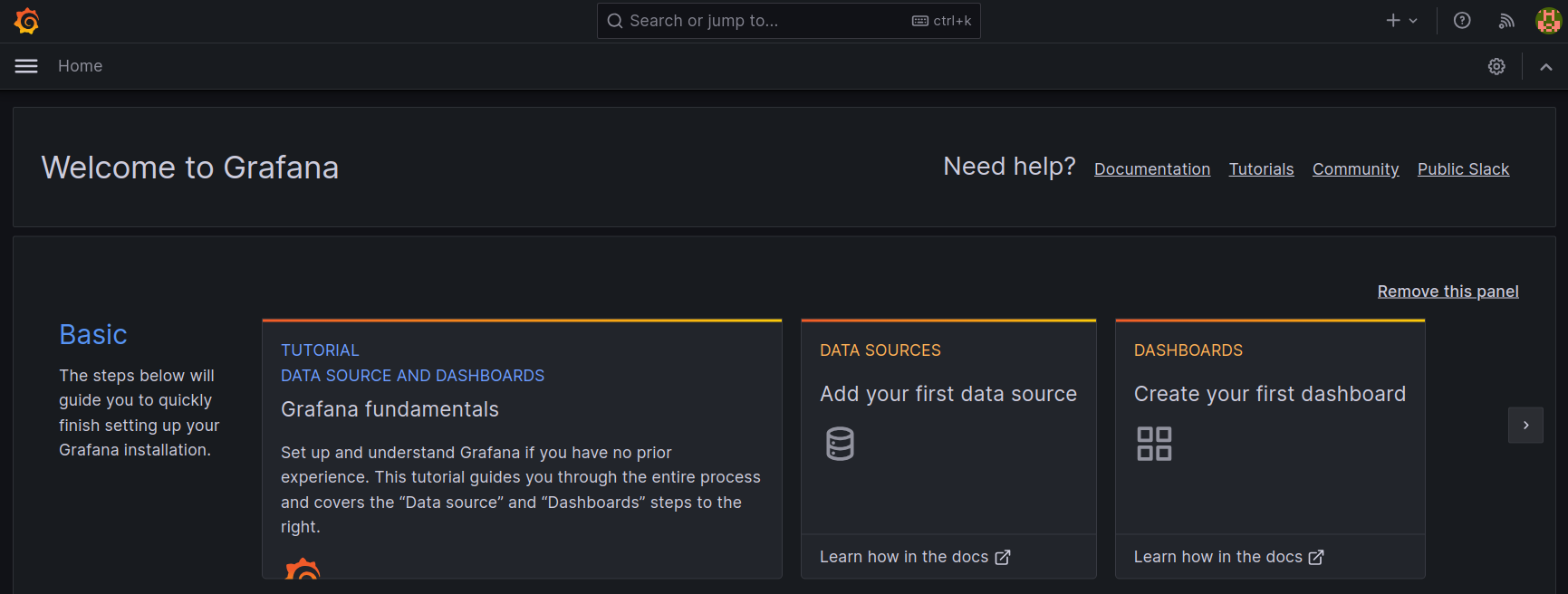
From the main page select the panel to add our first data source.
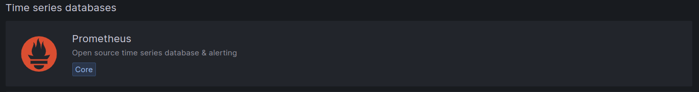
The select ‘Add Data Source’ and then select Prometheus as that data source.
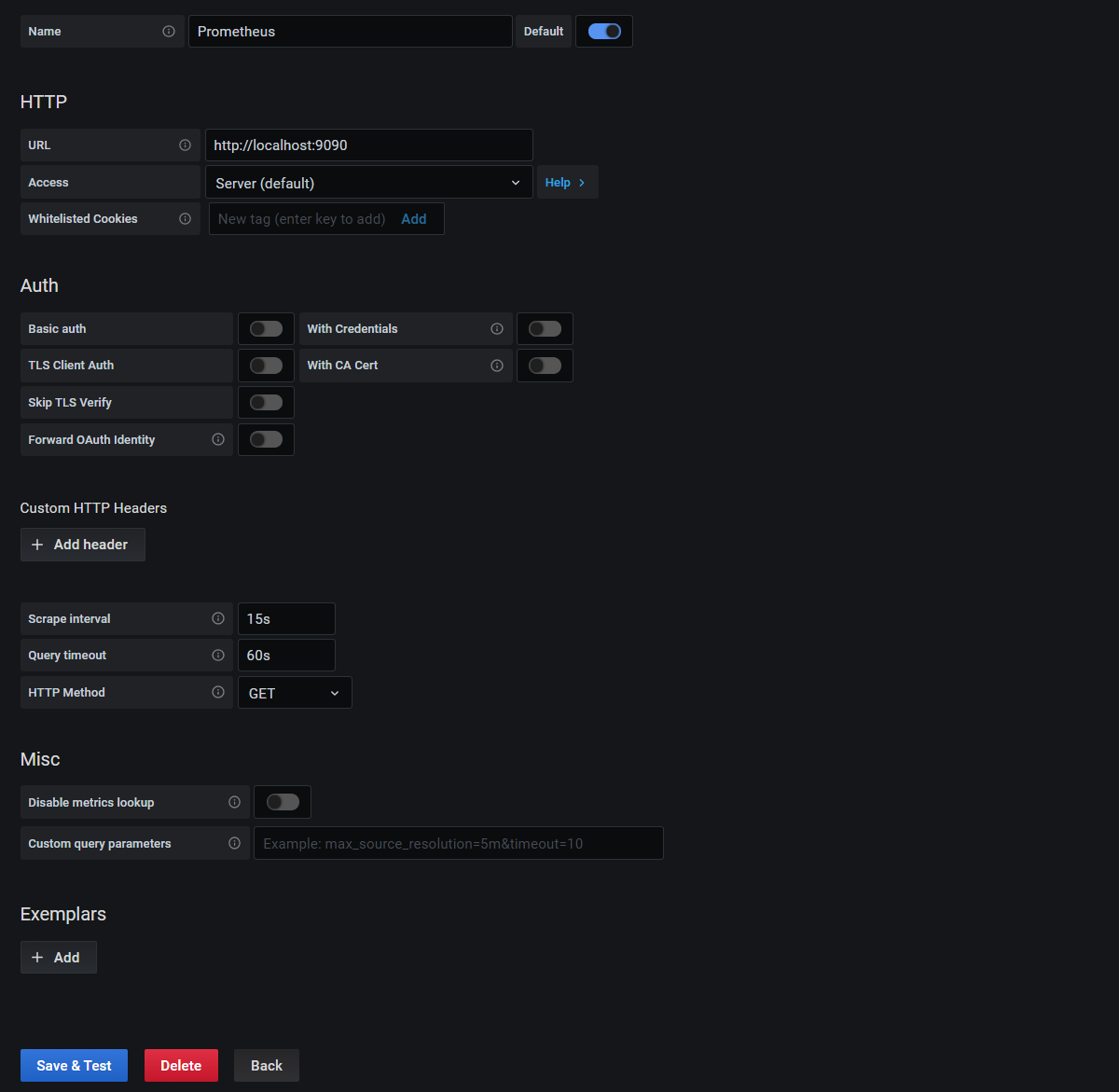
Now we get to configure some of the settings for our connection to Prometheus.
In this case we can set the URL as ‘http://localhost:9090’ (since both Prometheus and Grafana are installed on the same server), leave the scrape interval as ’15s’, the Query timeout as 60s and the http method as ‘GET’. Be aware that on some versions of Grafana, you will need to explicitly type in the URL ‘http://localhost:9090’ or you may receive an error when you test in the next step.
Then click on the ‘Save & Test button’.
We should get a nice tick to indicate that the data source is working.

Great!
Now things start to get just a little bit exciting. Remember the metrics that were being sent out by Prometheus? Those were the metrics that report back on how Prometheus is operating. In other words, it’s the monitoring system being monitored. We are going to use that to show our first dashboard.
Here lies another strength of Grafana. Dashboards can be built and shared by users so that everyone benefits. We will import one such dashboard to show us how Prometheus is operating.
At the top left of our page, click on the icon to return to the home screen.

There is a ‘Dashboards’ panel to create our first dashboard. Let’s click on that to show some available dashboards for our Prometheus instance;
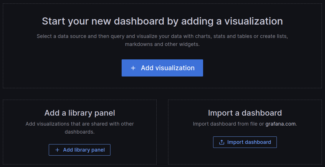
From here we can enter the Grafana dashboard ID number 3662 and click on the ‘Load’ button and then the ‘Import’ button.
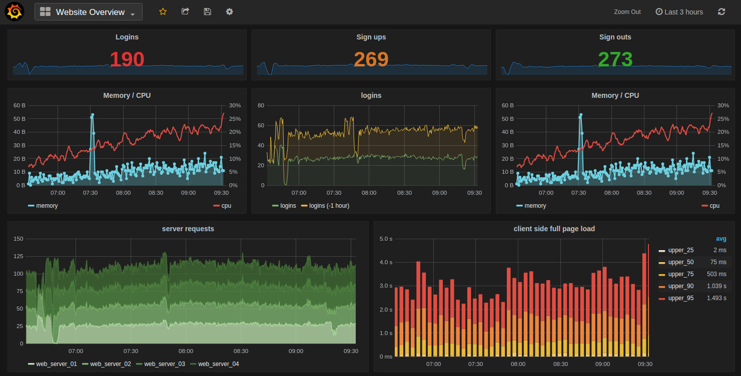
And the dashboard will open.
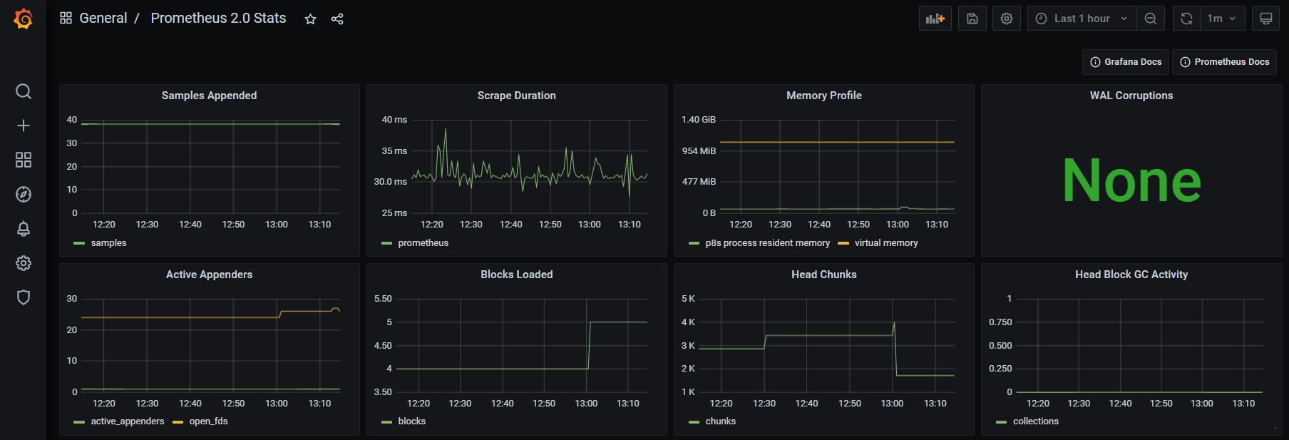
How about that?
We should now be looking at a range of metrics that Grafana is scraping from Prometheus and presenting in a nice fashion.
Trust me, this is just the start of our journey. As simple as the process of getting up and running and looking at a pretty graph is, there are plenty more pleasant surprises to come as we look at the flexibility and power of these two services.
Exporters
Gathering metrics in Prometheus involves pulling data from providers via agents called ‘exporters’. There are a wide range of pre-built exporters and a range of templates for writing custom exporters which will collect data from your infrastructure and send it to Prometheus.
Pre-built exporter examples include;
- Node Exporter: Which exposes a wide variety of hardware- and kernel-related metrics like disk usage, CPU performance, memory state, etcetera for Linix systems.
- SNMP Exporter: Which exposes information gathered from SNMP. Its most common use is to get the metrics from network devices like firewalls, switches and the devices which just supports SNMP only.
- Database Exporters: These are a range of exporters that can retrieve performance data from databases such as MySQL, MSSQL, PostgreSQL, MongoDB and more.
- Hardware Exporters: A number of hardware platforms have exporters supported including Dell, IBM, Netgear and Ubiquiti.
- Storage Platforms: Such as Ceph, Gluster and Hadoop
Custom exporter examples include libraries for Go, Python, Java and Javascript.
Node Exporter
As node_exporter is an official exporter available from the Prometheus site, and as the binary is able to be installed standalone the installation process is fairly similar. We’ll download it, decompress it and run it as a service.
In the case of the installation below the node_exporter will be installed onto another Raspberry Pi operating on the local network at the IP address 10.1.1.109. It will pull our server metrics which will be things like RAM/disk/CPU utilization, network, io etc.
First then we will browse to the download page here - https://github.com/prometheus/node_exporter/releases/. Remembering that it’s important that we select the correct architecture for our Raspberry Pi.
As the Pi that I’m going to monitor in this case with node_exporter uses a CPU based on the ARMv7 architecture, use the drop-down box to show armv7 options.
Note the name or copy the URL for the node_exporter file that is presented. The full URL in this case is something like - https://github.com/prometheus/node_exporter/releases/download/v1.3.1/node_exporter-1.3.1.linux-armv7.tar.gz;
Using a terminal, ssh into the node to be monitored. In our case, this swill be as the pi user again on 10.1.1.109.
Once safely logged in and at the pi users’s home directory we can start the download (remember, the command below will break across lines, don’t just copy - paste it);
The file that is downloaded is compressed so once the download is finished we will want to expand our file. For this we use the tar command;
Housekeeping time again. Remove the original compressed file with the rm (remove) command;
We now have a directory called node_exporter-1.3.1.linux-armv7. Again, for the purposes of simplicity it will be easier to deal with a directory with a simpler name. We will therefore use the mv (move) command to rename the directory to just ‘node_exporter’ thusly;
Again, now we need to make sure that node_exporter starts up simply at boot. We will do this by setting it up as a service so that it can be easily managed and started.
The first step in this process is to create a service file which we will call node_exporter.service. We will have this in the /etc/systemd/system/ directory.
Paste the following text into the file and save and exit.
The service file can contain a wide range of configuration information and in our case there are only a few details. The most interesting being the ‘ExecStart’ details which describe where to find the node_exporter executable.
Before starting our new service we will need to reload the systemd manager configuration again.
Now we can start the node_exporter service.
You shouldn’t see any indication at the terminal that things have gone well, so it’s a good idea to check node_exporter’s status as follows;
We should see a report back that indicates (amongst other things) that node_exporter is active and running.
Now we will enable it to start on boot.
The exporter is now working and listening on the port:9100
To test the proper functioning of this service, use a browser with the url: http://10.1.1.109:9100/metrics
This should return a lot lot statistics. They will look a little like this
Now that we have a computer exporting metrics, we will want it to be gathered by Prometheus
Prometheus Collector Configuration
Prometheus configuration is via a YAML (Yet Another Markup Language) file. The Prometheus installation comes with a sample configuration in a file called prometheus.yml (in our case in /home/pi/prometheus/).
The default file contains the following;
There are four blocks of configuration in the example configuration file: global, alerting, rule_files, and scrape_configs.
global
The global block controls the Prometheus server’s global configuration. In the default example there are two options present. The first, scrape_interval, controls how often Prometheus will scrape targets. We can still override this for individual targets. In this case the global setting is to scrape every 15 seconds. The evaluation_interval option controls how often Prometheus will evaluate rules. Prometheus uses rules to create new time series and to generate alerts. The global settings also serve as defaults for other configuration sections.
The global options are;
- scrape_interval: How frequently to scrape targets. The default = 1m
- scrape_timeout: How long until a scrape request times out. The default = 10s ]
- evaluation_interval: How frequently to evaluate rules. The default = 1m ]
- external_labels: The labels to add to any time series or alerts when communicating with external systems (federation, remote storage, Alertmanager)
alerting
The alerting section allows for the integration of alerts from Prometheus. In the default config above there are none set up and conveniently we are going to look at alerting from Grafana instead. So we can safely leave this alone.
rule_files
The rule_files block specifies the location of any rules we want the Prometheus server to load. For now we’ve got no rules. These recording rules allow Prometheus to evaluate PromQL expressions regularly and ingest their results. Recording rules go in separate files from our prometheus.yml file. They are known as rule files. We won’t be covering these in our examples in this book.
scrape_configs
The last block, scrape_configs, controls what resources Prometheus monitors. In our default case, only one scrape configuration exists that specifies a single job. In advanced configurations, this may be different. Since Prometheus also exposes data about itself it can scrape and monitor its own health. We can see that in the last line, - targets: ['localhost:9090']. In the default configuration there is a single job, called prometheus, which scrapes the time series data exposed by the Prometheus server. The job contains a single, statically configured, target, the localhost on port 9090. Prometheus expects metrics to be available on targets on a path of /metrics. So this default job is scraping via the URL: http://localhost:9090/metrics.
In our simplest means of adding metrics to Prometheus, we can add additional targets to this list.
Adding a monitoring node to Prometheus
In keeping with the information on the prometheus.yml file, we can simply add the IP address of a node that is running the node_exporter as a new target and we are good to go.
Let’s add the node that we configured in the previous section at 10.1.1.109.
At the end of the file add the IP address of our new node - targets: ['10.1.1.109:9100'];
Then we restart Prometheus to load our new configuration;
Now if we return to our Prometheus GUI (http://10.1.1.110:9090/targets) to check which targets we are scraping we can see two targets, including our new node at 10.1.1.109.
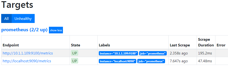
Let’s see our new node in Grafana!
Because we have already added Prometheus as a data source in Grafana, seeing or new node in a dashboard is ridiculously simple.
Go back to our Grafana GUI at http://10.1.1.110:3000.
Select the create icon which is the plus (‘+’) sign on the left hand side of the screen and then select ‘Import’.
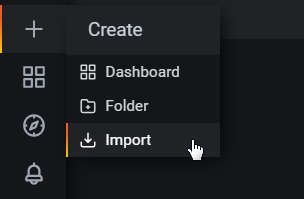
In the Grafana.com Dashboard box enter the dashboard number 1860 and then click on then ‘Load’ button.
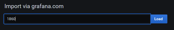
Under the prometheus Option use the drop-down arrow and select ‘Prometheus’.
Then click on ‘Import’.
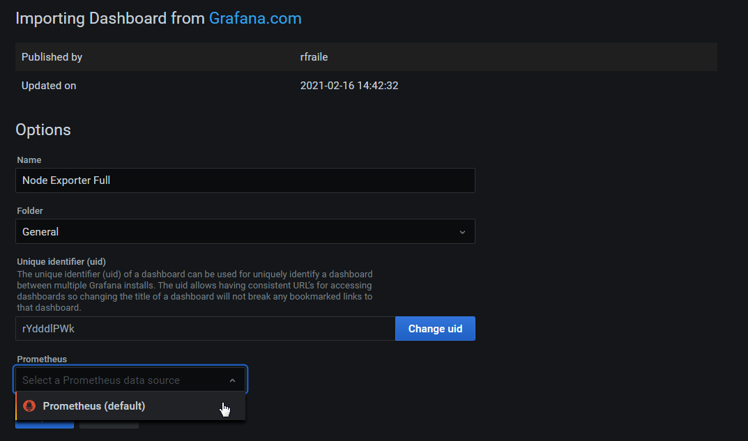
The dashboard should now be there in all its glory
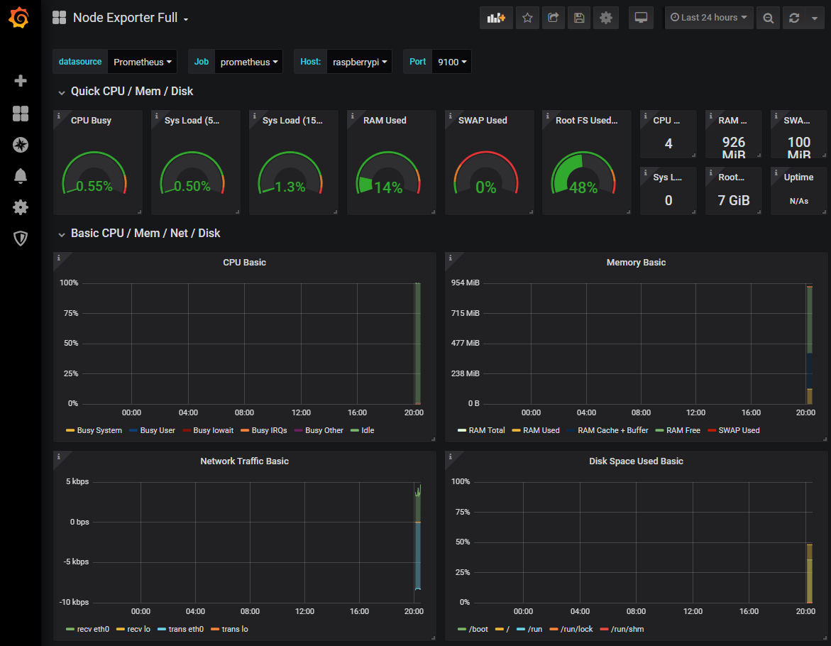
At this stage there probably won’t be much to see, but we can shorten the displayed time to the past 5 minutes by using the custom time range menu at the top right of the screen.
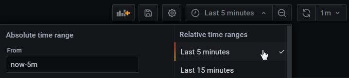
To keep the screen updating select the auto-refresh setting from the top right hand corner. In the screenshot below we are selecting 10 seconds.
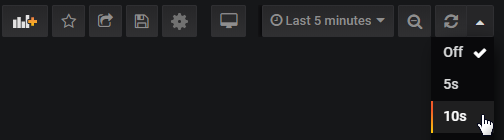
The end result is an automatically updating indication of the performance of our Raspberry Pi at 10.1.1.109.
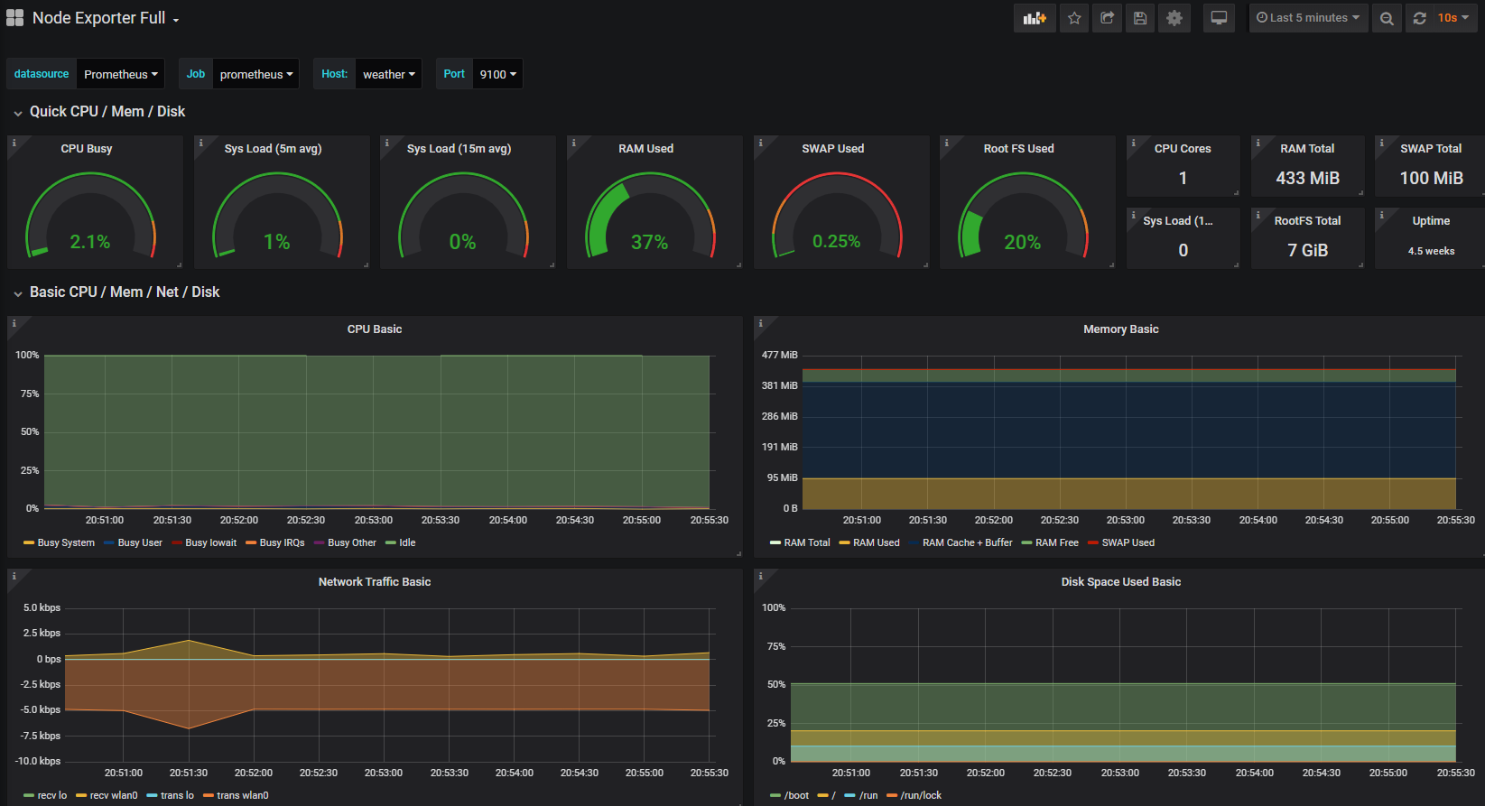
Take a few minutes to explore the additional panels at the bottom of the screen. This is a manifestation of the huge number of metrics that we saw in text form when we tested the scraping of the node_exporter installation, brought to life in graphical form.
WMI exporter
The node_exporter is ideal for gathering metrics on *NIX based systems, but Windows based systems will require a different exporter. The is where the WMI exporter comes in.
It has a wide range of collectors available and by default it will enable;
- CPU usage
- “Computer System” metrics (system properties, num cpus/total memory)
- Logical disks, disk I/O
- Network interface I/O
- OS metrics (memory, processes, users)
- Service state metrics
- System calls
- Read prometheus metrics from a text file
For this example we will make the assumption that the Windows computer has a IP address assigned. In the case for the example below the IP address we will be setting up and connecting to will be ‘10.1.1.99’.
Installing the WMI exporter
From the wmi_exporter releases page, download the appropriate installer for your system.
Run the file (the sequence below illustrates using the amd64 msi and version v0.11.0)
We will be asked for verification;
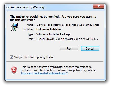
And then the program is configured;
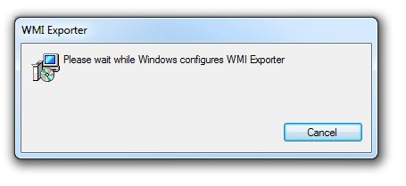
We also need to let the program make changes to the computer;
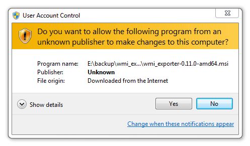
We should now have the WMI exporter service running as a service on our Windows computer.
We can test this (on the Windows machine) by entering the local address (http://localhost:9182/metrics) into a web browser (The default port for wmi_exporter is 9182). This should produce a nice long list of metrics something like the following;
# HELP go_gc_duration_seconds A summary of the GC invocation durations.# TYPE go_gc_duration_seconds summarygo_gc_duration_seconds{quantile="0"} 0go_gc_duration_seconds{quantile="0.25"} 0go_gc_duration_seconds{quantile="0.5"} 0go_gc_duration_seconds{quantile="0.75"} 0.001go_gc_duration_seconds{quantile="1"} 0.001go_gc_duration_seconds_sum 0.002go_gc_duration_seconds_count 8# HELP go_goroutines Number of goroutines that currently exist.# TYPE go_goroutines gaugego_goroutines 13# HELP go_info Information about the Go environment.# TYPE go_info gaugego_info{version="go1.13.3"} 1Adding adding our Windows exporter to Prometheus
Just as we did with the node_exporter we need to add the IP address of our new metrics source (10.1.1.99) to the Prometheus prometheus.yml file. To do this we can simply add the IP address of our computer that is running the wmi_exporter as a new target with the default port (9182) and we are good to go.
On our Prometheus server;
At the end of the file add the IP address of our new node - targets: ['10.1.1.99:9182'];
Then we restart Prometheus to load our new configuration;
Now if we return to our Prometheus GUI (http://10.1.1.110:9090/targets) to check which targets we are scraping we can see three targets, including our new node at ‘10.1.1.99:9182’.

Let’s see our new node in Grafana!
Go back to our Grafana GUI at http://10.1.1.110:3000.
Select the create icon which is the plus (‘+’) sign on the left hand side of the screen and then select ‘Import’.
Here we will follow the same process to import a pre-prepared desktop for Windows host metrics. In the Grafana.com Dashboard box enter the dashboard number 10171.
After going through the process our new dashboard should now be there in all its glory
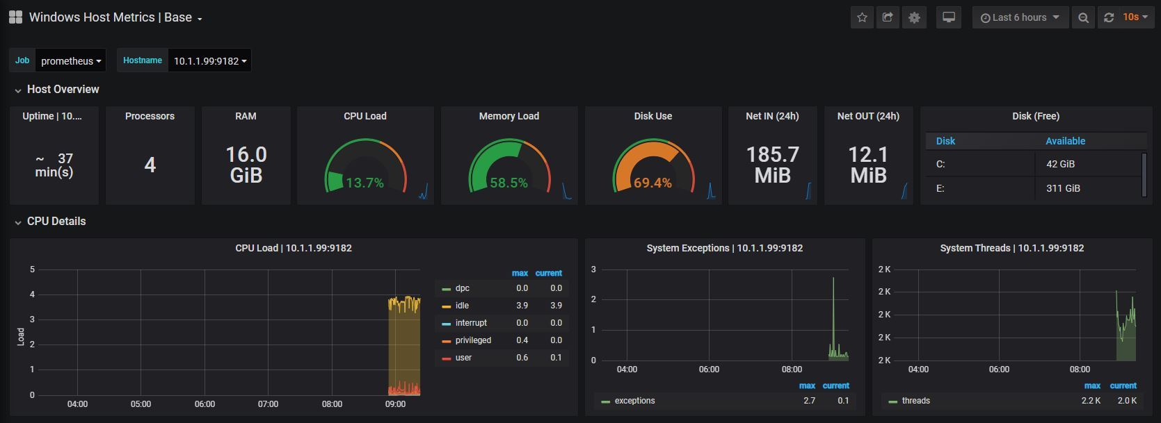
At an early stage there probably won’t be much to see, but take a few minutes to explore the additional panels at the bottom of the screen. This is a manifestation of the huge number of metrics that we saw in text form when we tested the scraping of the wmi_exporter installation.
Custom Exporters
As much as the available information from node_exporter is extraordinary, if you have developed a project or need to monitoring something unique, you will want to integrate it with Prometheus / Grafana. This is where custom exporters come in.
The process is described as ‘instrumentation’. In the sense that it’s like adding sensors to different parts of your system that will report back the data your looking for. The same way developers of high performance vehicles will add measuring instruments to gauge performance.
We can add this instrumentation via client libraries that are supported by Prometheus or from a range of third party libraries. The officially supported libraries are;
- Go
- Java or Scala
- Python
- Ruby
When implemented they will gather the information and expose it via a HTTP endpoint (the same way that node_exporter does with http://<IP Address>:9100/metrics.
In the example that we will develop we will collect information from a platform that is measuring the depth of water in a tank and the temperature of the water and we will use the Python client library. Readers of some of my other books may recognise that as the data that I describe measuring in Raspberry Pi Computing: Ultrasonic Distance Measurement and Raspberry Pi Computing: Temperature Measurement.
Metrics
We could easily cut straight to the code and get measuring, (and feel free to do that if you would prefer) but it would be useful to learn a little about the different metric types available and some of the ways that they should be implemented to make the end result integrate with other metrics and follow best practices for flexibility and efficiency.
Metric Types
Prometheus recognises four different core metric types;
- Counter: Where the value of the metric increments
- Gauge: Where the metric value can increase or decrease
- Histogram: Where values are summed into configurable ‘buckets’.
- Summary: Similar to the Histogram type, but including a calculation of configurable quantiles.
Metric Names
Prometheus is at heart a time series recording platform. To differentiate between different values, unique metric names are used.
A metric name should be a reflection of the measured value in context with the system that is being measured.
Metric names are restricted to using a limited range of ACSII letters, numbers and characters. These can only include a combination of;
- a through z (lowercase)
- A through Z (uppercase)
- digits 0 through 9
- The underscore character (_)
- The colon (:)
In practice, colons are reserved for user defined recording rules.
Our metric names should start with a single word that reflects the domain to which the metric belongs. For example it could be the system, connection or measurement type. In the metrics exposed by node_exporter we can see examples such as ‘go’ for the go process and ‘node’ for the server measurements. For our two measurements we are measuring different aspects of the water in the water tank. Therefore I will select the prefix ‘water’
The middle part of name should reflect the type of thing that is being measured in the domain. You can see a range of good examples in the metrics exposed from our node_exporter. For example ‘cpu_frequency’ and ‘boot_time’. For our measurements we would have ‘depth’ and ‘temperature’.
The last part of the name should describe the units being used for the measurement (in plural form). In our case the water depth will be in ‘metres’ and the temperature will be in ‘centigrade’
The full name of our metrics will therefore be;
- water_depth_metres
- water_temperature_centigrade
Metric Labels
Metric labels are one of the features of Prometheus that allow dimensionality. for example a multi-core CPU could have four metrics with identical names and labels that differentiated between each core. For example;
- node_cpu_frequency_hertz{cpu=”0”}
- node_cpu_frequency_hertz{cpu=”1”}
- node_cpu_frequency_hertz{cpu=”2”}
- node_cpu_frequency_hertz{cpu=”3”}
In our example there is a possibility that we will be measuring water temperature in different locations and therefore we might see;
- water_temperature_centigrade{location=”inlet”}
- water_temperature_centigrade{location=”solar”}
- water_temperature_centigrade{location=”outlet”}
This will be true for another project that I intend to complete, therefore I will add a label to this metric with the knowledge that it will give me the ability to easily compare between a range of water temperature measurements from around the house. This metric will therefore be
- water_temperature_centigrade{location=”tank”}
As with metric names we are restricted as to which ASCI characters we can use. This time we aren’t allowed to use colons so the list is;
– a through z (lowercase) - A through Z (uppercase) - digits 0 through 9 - The underscore character (_)
We won’t be starting our metric values with an underscore as these are reserved for internal use.
We can have multiple labels assigned to a metric. Simply separate them with a comma.
Configuring the exporter
To use the custom exporter on our target machine (in this case the IP address of the Pi on the water tank is 10.1.1.160), we’ll need to install the Prometheus client library for Python and pip as follows;
To collect information, we need to make sure that we can gather it in a way that will suit our situation. In the system that we will explore, our temperature and distance values are read by Python scripts that are run by cron jobs every 5 minutes. We could use those same scripts in our custom exporter, but in this case, the act of taking the measurement actually takes some time and our running of the custom exporter might interfere with the running of the cron job (in other words two scripts could be trying to operate a single physical sensor at the same time).
To simplify the process I have added a small section to the scripts that read the depth of the water and the temperature of the water. Those sections simple write the values to individual text files (distance.txt and temperature.txt) that can then be easily read by out exporter. This techniques has pros and cons, but for the purpose of demonstrating the collection written the technique is simple and adequate.
As an illustration, the following is the code snippet that is in the temperature measuring script;
  # write the temperature value to a file
  f = open("temperature.txt", "w")
  f.write(str(temperature)[1:-1])
  f.close()
There is a variable, temperature already in use (having just been recorded by the script). The file name ‘temperature.txt’ is opened as writeable, the value is written to the file (the leading and trailing character is removed by the [1:-1] because strings/numbers), overwriting the previous value and the file is closed.
Meanwhile, our python exporter script which in this case is named tank-exporter.py looks like the following;
import prometheus_client
import time

UPDATE_PERIOD = 300

tank_depth = prometheus_client.Gauge('water_depth_metres',
                              'Depth of water in water tank. Full = 2.7m',
                              ['location'])
water_temperature = prometheus_client.Gauge('water_temperature_centigrade',
                              'Temperature of water in water tank',
                              ['location'])

if __name__ == '__main__':
  prometheus_client.start_http_server(9999)

while True:
  with open('/home/pi/distance.txt', 'r') as f:
      distance = f.readline()

  with open('/home/pi/temperature.txt', 'r') as g:
      temperature = g.readline()

  tank_depth.labels('water_tank').set(distance)
  water_temperature.labels('water_tank').set(temperature)
  time.sleep(UPDATE_PERIOD)
The main actions in our exporter can be summarized by the following entries:
- Import the Prometheus client Python library.
- Declare two gauge metrics with the metric names that we developed earlier.
- Instantiate an HTTP server to expose metrics on port 9999.
- Start a measurement loop that will read our metric values every 5 minutes
- Gather out metric values from our text files.
- The metrics are declared with a label (location), leveraging the concept of multi-dimensional data model.
In the same way that we made sure that node_exporter starts up simply at boot, we will configure our Python script as a service and have it start at boot.
The first step in this process is to create a service file which we will call tank_exporter.service. We will have this in the /etc/systemd/system/ directory.
Paste the following text into the file and save and exit.
The service file can contain a wide range of configuration information and in our case there are only a few details. The most interesting being the ‘ExecStart’ details which describe where to find python and the tank-exporter.py executable.
Before starting our new service we will need to reload the systemd manager configuration again.
Now we can start the tank_exporter service.
You shouldn’t see any indication at the terminal that things have gone well, so it’s a good idea to check tank_exporter’s status as follows;
We should see a report back that indicates (amongst other things) that tank_exporter is active and running.
Now we will enable it to start on boot.
The exporter is now working and listening on the port:9999
To test the proper functioning of this service, use a browser with the url: http://10.1.1.160:9999/metrics
This should return a lot lot statistics. They will look a little like this
There are a lot more metrics than just out water tank info, but you can see our metrics at the top.
Now that we have a computer exporting metrics, we will want it to be gathered by Prometheus
Adding adding our custom exporter to Prometheus
Just as we did with the node_exporter we need to add the IP address of our new metrics source to the Prometheus prometheus.yml file. To do this we can simply add the IP address of a node that is running the septic_exporter as a new target and we are good to go.
On our Prometheus server;
At the end of the file add the IP address of our new node - targets: ['10.1.1.160:9999'];
Then we restart Prometheus to load our new configuration;
Now if we return to our Prometheus GUI (http://10.1.1.110:9090/targets) to check which targets we are scraping we can see three targets, including our new node at 10.1.1.160.
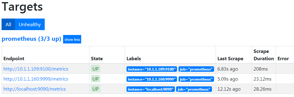
Creating a new graph in Grafana
Righto…
We now have our custom exporter reading our values successfully, let’s visualize the results in Grafana!
From the Grafana home page select the Add icon (it’s a ‘+’ sign) from the left hand menu bar and from there select dashboard. Technically this is adding a dashboard, but at this stage we’re just going to implement a single graph.
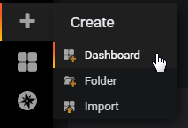
The next screen will allow us to start the process by either choosing the type of visualisation (Line graph, gauge, table, list etc) or by simply adding a query. In our case we’re going to take a simple route and select ‘Add Query’. Grafana will use the default visualisation which is the line graph.
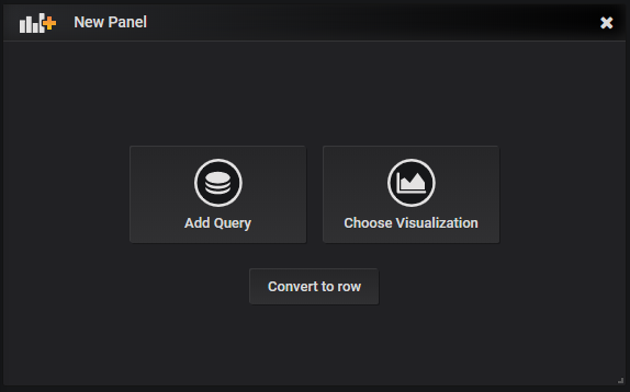
Now we are presented with our graph with no data assigned.
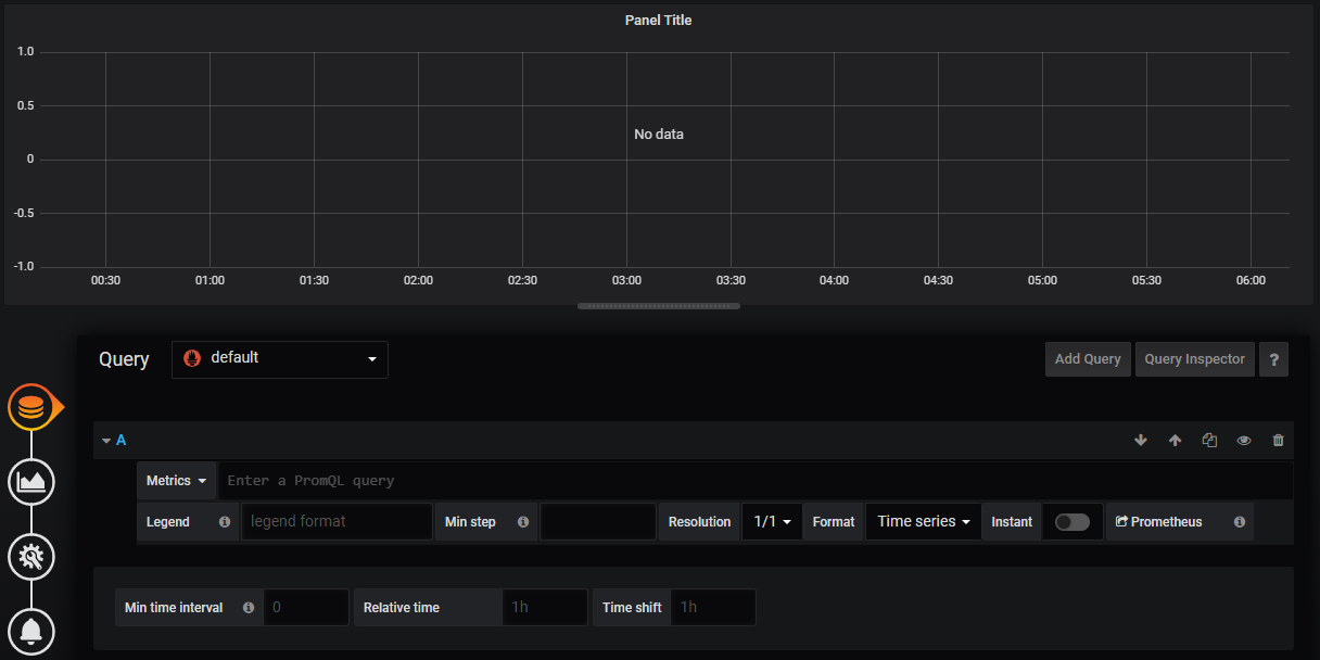
By adding a query, we are selecting the data source that will be used to populate the graph. The main source that our Query will be selecting against is already set as the default Prometheus. All that remains for us is to select which metric we want from Prometheus.
We do that by clicking on the ‘Metrics’ drop down which will provide a range of different potential sources. Scroll down the list and we will see ‘water’ which is the first part of our metric name (the domain) that we assigned. Click on that and we can see the two metrics that we set up to record. Select ‘water_depth_metres’.
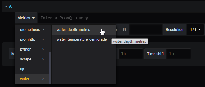
That will instantly add the metric data stream with whatever data has been recorded up to that point. Depending on how fast you are, that could be only a few data points or, as you can see from the graph below, there could be a bit more.
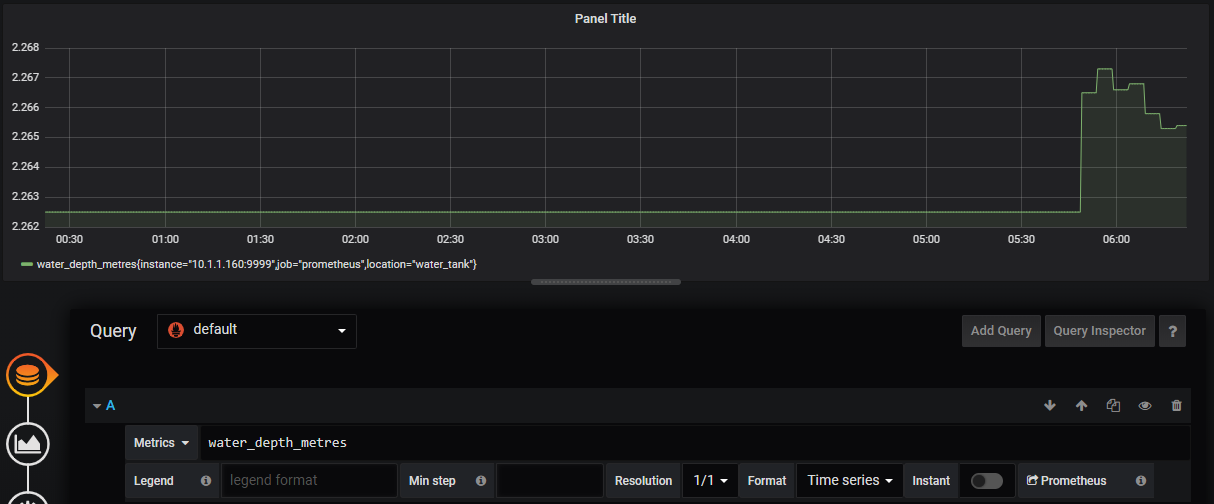
Spectacularly we have our graph of water depth!
At the moment it’s a static graph, so let’s change it to refresh every minute by selecting the drop-down by the refresh symbol in the top right corner and selecting ‘1m’.
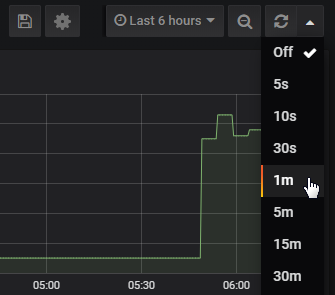
Now all we have remaining is to save our masterpiece so that we can load it again as desired. To do this, go to the save icon at the top of the screen and click it.
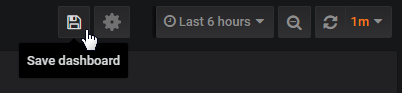
The following dialogue will allow us to give our graph a fancy name and then we slick on the ‘Save’ button.

There it is! It looks slightly unusual stuck on the left hand side of the screen, but that’s because it is a single graph (or panel) in a row that is built for two. As an exercise for the reader, go through the process of adding a second panel by selecting the ‘Add Panel’ icon on the top of the screen.

This time select the water temperature as the metric. You might want to move the panel about to get it in the righ place and you can adjust the size of the panels by grabbing the corners of the individual panels. Ultimately something like the following is the result!
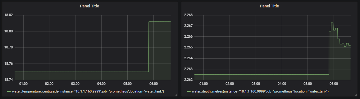
Not bad for a few mouse clicks. Make sure that you save the changes and you’re done!
Dashboards
A dashboard is at the heart and soul of a monitoring system. There are plenty of other seriously important aspects, but as human beings, we have a considerable talent for considering a great deal of information quickly from an image. The key with doing that effectively is to present the information in a way that is logical and provides clarity to the data.
Overview
One of Grafana’s significant strengths is its ability to be able to present data in a flexible way. The support for adding different ways of illustrating metrics and for customising the look and feel of those visualisations is one of the defining advantages to using Grafana and a reason for its popularity.
In this section we will look at the individual panels that are used to build dashboards and how they might be employed for best effect.
New Panel
To start the process of creating our own dashboard we need to use the create menu from the left hand side of the screen (it’s a plus (‘+’) sign).
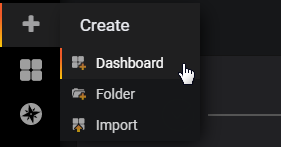
That will then give us the potion of starting the process of sorting out our data and then worrying about the visualisation method or choosing the visualisation method and then assigning the data. Both methods are valid for different situations, but for the sake of demonstrating different options for maximum effect, let’s take a look at the visualisation options. From the new panel window choose ‘Add Query’
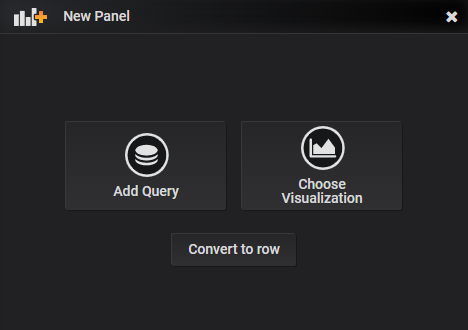
Each panel has up to four different configuration options depending on the visualisation type selected
- Query: Where our data source can be specified and adapted for our use
- Visualization: Where we select from the range of panel options
- General: For applying a custom title to the panel and linking to other panels
- Alerts: where we can set up alerts for notifications
Query Options
If we start from the ‘Query’ section, there will be a default graph type placed on the screen for the sake of having something there that will show some graphical goodness.
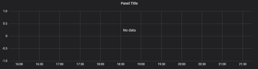
Our query options are shown directly underneath and represent our doorway to our data sources
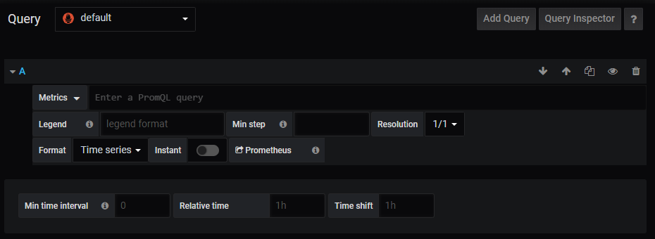
The default source in this case is Prometheus and it has already been selected.
We can add several different queries to a panel which is why there is an ‘A’ at the start of the options. Directly under this is our ‘Metrics’ drop-down menu. To put something interesting on the screen, select ‘metrics > prometheus > prometheus_http_requests_total’.
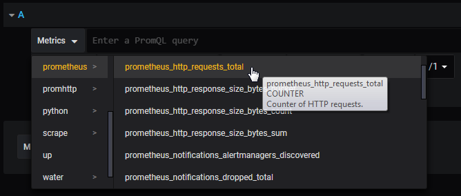
This will (depending on how long our instance of Prometheus and Grafana have been running) show some nice looking lines in our default panel above our query.
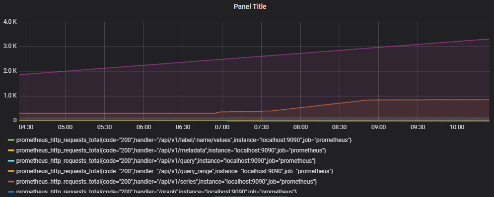
This graph is showing us the number of http requests that have been accumulating. This in turn has been broken down according to the code, handler, instance and job which we can see under the graph.
Now, this additional information is one of the strengths of Grafana. By asking for a particular metric, we have a number of data series that can be used in comparison. Alternatively, we might want to narrow down what we see via our query.
For example, if we wanted to just see http requests that were associated with the ‘/api/v1/query_range’ handler we would change our query from;
… to …
We will notice as we type in the curly brackets in the query box, Grafana helps out by showing the options we have to select from.
This then leaves us with a graph with only two lines on it;
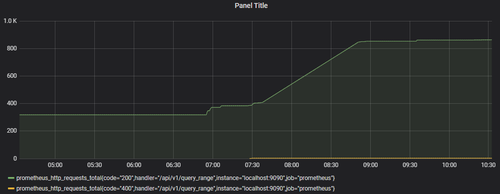
If we wanted to go further, we could filter by an additional label by separating our ‘handler’ qualifier from an additional one with a comma. Eg;
The query options are very powerful for selecting, adapting and filtering the information that we want to see.
Visualization Options
Selecting ‘Visualization’ will start the process of creating a panel by choosing the type of graphical display. The default that will come up is the traditional ‘Graph’.
Under this is the range of current (as of version 6.6.0) visualisation options.
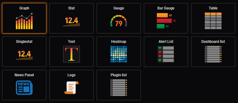
They represent;
- Graph: A traditional line / bar / scatterplot graph.
- Stat: Displays a single reading and includes a sparkline
- Gauge: A single gauge with thresholds
- Bar Gauge: A space efficient gauge using horizontal or vertical bars
- Table: Shows multiple data points aligned in a tabular form
- Singlestat: Displays a single reading from a metric
- Text: For displaying textural information
- Heatmap: Can represent histograms over time
- Alert List: Shows dashboard alerts
- Dashboard List: Provides links to other dashboards
- News Panel: Shows RSS feeds
- Logs: Show lines from logs.
- Plugin List: Shows the installed plugins for our Grafana instance
Graph
As we discussed earlier, the ‘Graph’ panel is the default starting point when selecting ‘Choose Visualisation’ from the panel menu. I think that it’s fair to say that there’s a good reason for that. Time series data is well suited to this form of display and the Graph panel provides plenty of options for customisation.
To get a feel for the different Graph options we need to load some data via the query menu (I know that this seems like perhaps we should have selected ‘Add Query’ first, but how else would we have looked at all the pretty panel option icons?)
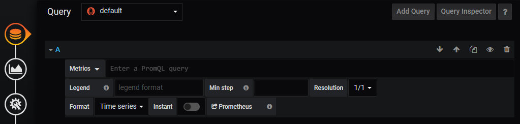
Click on the ‘Metrics’ menu and select something appropriately interesting looking. In my case I’ve picked ‘Weather -> weather_outside_temperature_C’
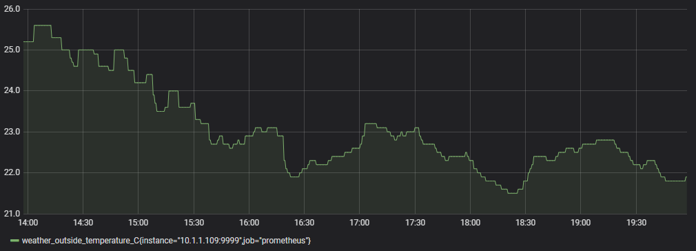
And there is our graph! It really is pretty easy.
Take a moment to experiment with the query options under the graph.
Now go back to the Visualisation menu. With some data we can now see the impact of experimenting with the controls for changing the appearance of the graphs.
Look at the ‘Draw Modes’. This will allow us to transform between the line graph that we already have to bars or points.
In the ‘Axes’ section change the ‘Mode’ for the ‘X-Axis’ from ‘Time’ to ‘Histogram’ to ‘Series’ this provides options for binning data depending on different dimensions.
Also have a look at the ‘Thresholds & Time Regions’ section. Here we can provide some useful context for the audience as to what expected operational limits might be.
The example below has set thresholds for acceptable, operation. Above 24 is a warning, above 25 is critical. Below 23 is also a warning and below 22 is critical.
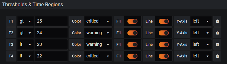
Sure, it’s contrived in our example, but it illustrates the usefulness of the option.
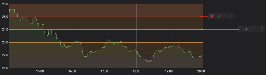
Stat
The ‘Stat’ panel is intended to replace the ‘Singlestat’ panel. The reason for this is that it has been built with integrated features that tie in the overall infrastructure for Grafana and maintains a common option design.
It is primarily designed to display a single statistic from a series. This could be a maximum, minimum, average or sum of values, or indeed the latest value available.
We will demonstrate useful features of the visualisation type by adding a stat panel to display temperature.
To make a start I have selected a data source query that shows inside temperature from a weather station.
From here select the ‘Stat’ visualisation type.
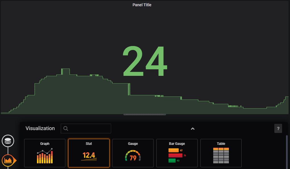
Automatically we can see that our display shows a prominent value for our panel and a representative ‘sparkline’ as an indication of the metrics change over time.
We can see from the ‘Display’ options that the value presented is the mean of the metrics. If we wanted to show some other option there we could select something like min, max or latest (i.e, what it the temperature now). I’m more interested in the current temperature, so will select ‘Last’.
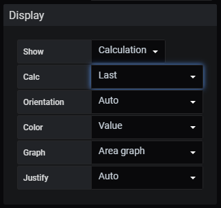
From the ‘Display’ options we can also turn off the background graph if desired as well as several other features.
The Field option will allow us to add units to our value and to get a little more granularity by showing how many decimal places we want to show.
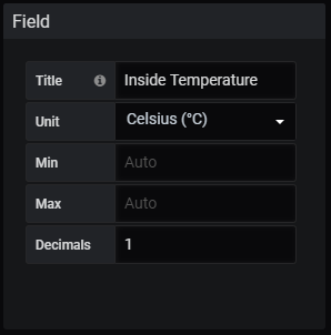
Thresholds are a great way to provide more context for our visualisation. In this instance I’d like to show the figure as red if the temperature is below 10 degrees or above 30 degrees
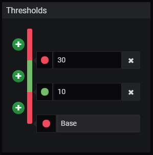
As an alternative to the thresholds, we could use value mapping to convert any temperature above 30 degrees to the text ‘Too Hot’ using the ‘Value mappings’ option;
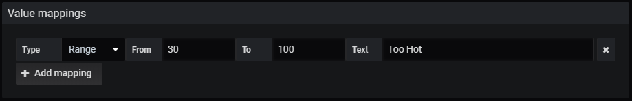
From the ‘General options tab / icon we can change the title of our panel to something appropriate.
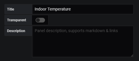
Save our dashboard and we’re done!
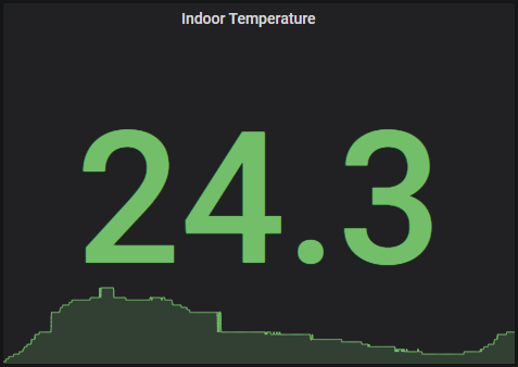
Gauge
The gauge visualization is a form of singlestat with the addition of a visualisation of the value presented in context with expected limits.
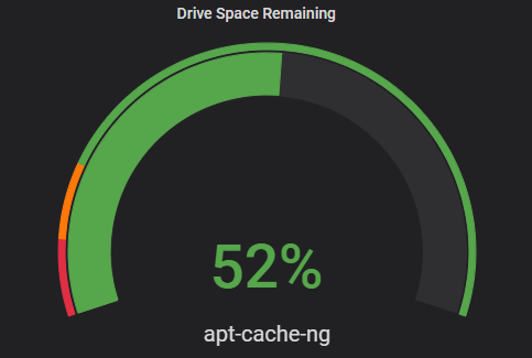
In the gauge example above we are presented with the amount of drive space remaining on the apt-cache-ng server where there are limits set to denote warning and critical values.
The example is derives from the metrics sourced from the node_exporter exporter on a server.
In this case, because we want to present a percentage of free space we need to know what the amount of space available is and the amount of space free.
Luckily, node_exporter has just those metrics available as node_filesystem_size_bytes and node_filesystem_avail_bytes. So while the visualisation type will be gauge, the first thing we really want to do is to establish our query.
In the query menu option area, we will be using a query that will take the form of 100 * (available space / total space)
This will look something like the following (it should be one contiguous line, but I have placed it across different lines here to prevent random line-breaks);
100*(
  node_filesystem_avail_bytes{fstype="ext4",instance="10.1.1.16:9100"}
  /
  node_filesystem_size_bytes{fstype="ext4",instance="10.1.1.16:9100"}
)
As astute readers you will also have noticed that I have narrowed down the returned data so that is only includes one device (via the IP address) and only for one file system type (ext4). This will return only a single graph of our desired server. Alternatively, by removing the ‘instance-"10.1.1.19:9100"’ we can show the remaining space in all the servers that we are monitoring;
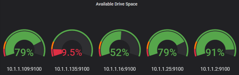
In the ‘Visualization’ options area, we will want to make sure that we display the last reading;
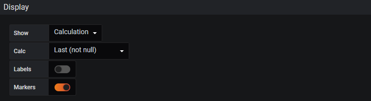
We will also provide a title to our gauge so that we know what the reading is associated with and we will assign it a unit of ‘percent’.
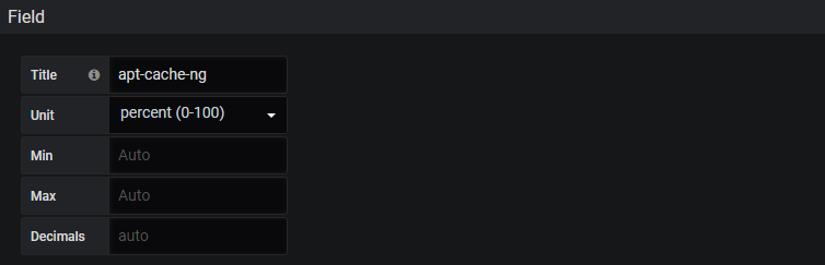
Finally we will set some thresholds that will provide a clear indication when the percentage of available storage has fallen below levels that we might deem acceptable.
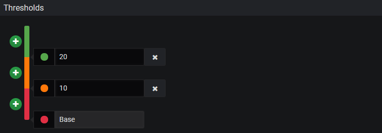
Above we can see that anywhere from our base value (which for the units of percentage is 0) to 10% will be red. Between 10 and 20 we will represent it as orange and between 20 and 100 (again, the percentage units help out) we will have green.
Bar Gauge
The bar gauge is almost a duplication of the gauge visualisation, with the exception that there are some different options available to represent the bars.
In the same way that we represented multiple gauges in the ‘Gauge’ example, our bar gauge will show an arguably more compact variation of the same principle. The example is the default ‘Retro LCD’ mode.
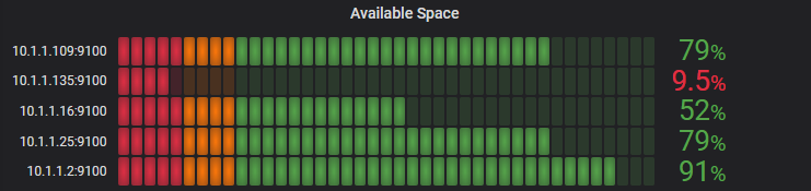
Alternative modes are gradient;
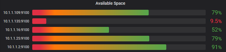
… and ‘Basic’
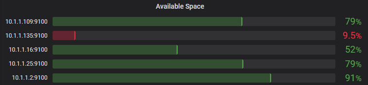
Any one of which would be acceptable.
Table
The ‘Table’ panel allows for the visualisation of time series information and log / event date in a table format. This allows for a better view of the exact value of data points in a series at the expense of providing a view of larger amounts of data or trends over longer periods of time.
Individual cells for the table can be coloured depending on the value of the displayed metric.
Singlestat
The ‘Singlestat’ visualisation is a legacy version of the ‘Stat’ visualisation. They are able to produce pretty much the same display, but go about it in slightly different way. The good folks at Grafana have said that the ‘Stat’ visualization is the way forward, so opt for that.
Text
The ‘Text’ panel allows us to add fixed textural information that can be useful for dashboard users.
Heatmap
‘Heatmap’s as implemented in Grafana provide the facility to view changes in a histogram over time.
Dashboard List
The ‘Dashboard List’ panel is an area that provides the ability to display links to other dashboards. The displayed list can be in the form of dashboards that have been ‘starred’ as a favourite or recently viewed. It can also employ a search element.
News Panel
We can add our favourite RSS feeds as a panel. There may be problems satisfying CORS restriuctions, in which case it is possible to use a proxy.
For example, if the BBC feed at http://feeds.bbci.co.uk/news/world/rss.xml didn’t work we can add a proxy to the front such as https://cors-anywhere.herokuapp.com/http://feeds.bbci.co.uk/news/world/rss.xml
Logs
A ‘Logs’ panel can display log entries from data sources such as Elastic, Influx, and Loki. It is possible to use the queries tab to filter the logs shown or to include multiple queries and have then merged.
General
If we go down to the ‘General’ menu we can see the option to change the title of our graph.

Alerting
If you quickly click along the list of different visualisation types, you will notice that the ‘Graph’ panel has one particular difference to all the others. The menu options down the left hand side include one option that is unique. The ‘Alert’ option.
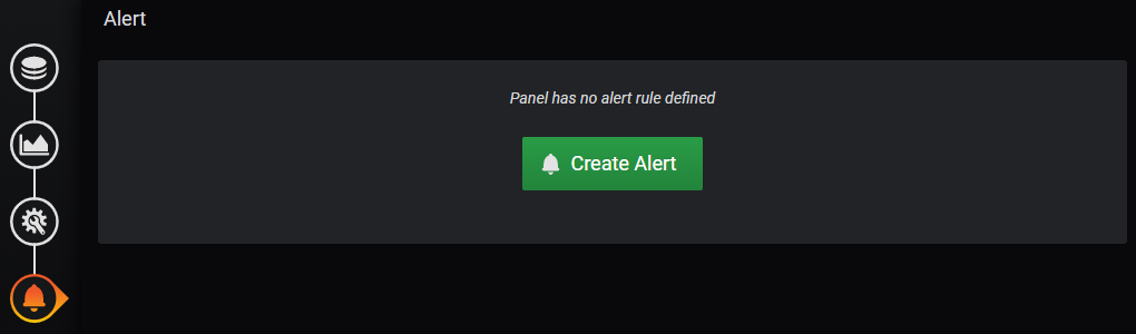
Alerts allow us to set limits on our graphs such that when they are exceeded, we can send out notifications (we could for instance have one that indicated a drop in temperature that sent an alert to let you know to cover up delicate seedlings or an increase in used disk space that indicated a problem on a computer.
Looking at a graph of data that represents the depth of water in a water tank, let’s step through the process of initiating an alert if the water depth goes below 1m.
First we would click on the ‘Create Alert’ button.
This then allows us to set up our rule and the conditions under which it can alert.
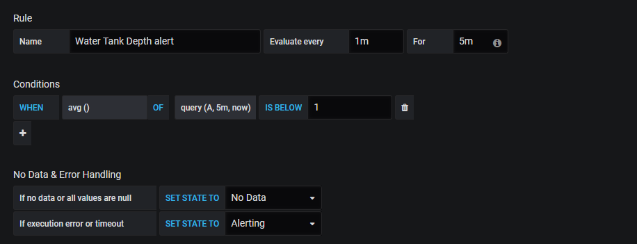
The image above shows that the water depth will be every minute for 5 minutes. That means that Grafana will look for the condition every minute. If our condition is violated for 5 consecutive minutes it will have been adjudged as having met the threshold for sending a notification.
Under that we can see the condition being set as the average of the readings in the last 5 minutes being less than 1 metre.
Now we’ll need to do a bit of behind the scene configuration
To enable email notifications we will edit a config file. It will be in different places or even named differently depending on how you installed Grafana. If we had done so via a deb or rpm package it would be at /etc/grafana/grafana.ini. However, as we installed it as a pre-prepared binary it is in the grafana directory in our home directory and in this case as it is a pretty clean stock install I’m going to use the defaults.ini file.
Open the file and in the ini file change the SMTP area change the settings to something like the following using your username and password details. The below settings are for a Gmail notification and as such others will differ. For a Gmail account, to make life a little easier (and less secure -Beware! - ) you will want to set your account to allow less secure apps and to disable 2 factor authentication.
#################################### SMTP / Emailing #####################[smtp]enabled = truehost = smtp.gmail.com:587user = somepiuser# If password contains # or ; wrap it in triple quotes. """#password;"""password ="""mypassword"""cert_file =key_file =skip_verify = falsefrom_address = admin@grafana.localhostfrom_name = Grafanaehlo_identity =[emails]welcome_email_on_sign_up = falsetemplates_pattern = emails/*.html
For this to take effect we need to restart Grafana;
Now we want to set up a new notification channel.
From our alerting menu (look for the ‘bell’ icon), select ‘Add Channel’;
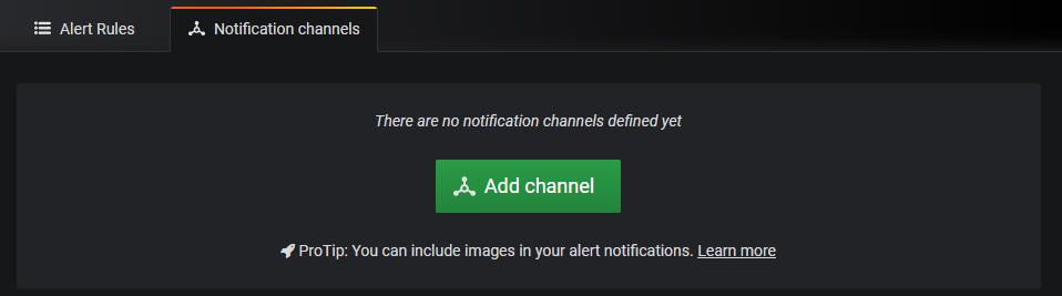
Now we can configure our notification channel. In the case below we are sending an email to the address that is blurred out and the name of the channel is ‘Gmail Alert’
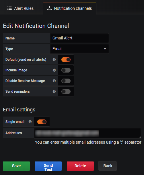
It’s a good idea to test that it works and you can do that from here using the ‘Send Test’ button.
If things don’t go well for the test, check out syslog (/var/log/syslog) for clues to the error.
Then we can set the notification in our graph panel.
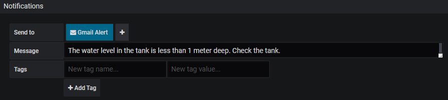
We can see that our ‘Gmail Alert’ notification is selected. We have also set a message to be sent to tell us that the water is too low.
Upgrading Prometheus
Upgrading Prometheus is something that we should do as new versions with new features become available. Because we have installed our system by downloading and running is as a standalone binary, the simple method such as using the apt-get track won’t work for us.
However, that doesn’t mean that it’s a difficult task. In fact, it’s blissfully easy.
We can make the process fairly straight forward and painless by installing the new version alongside our older version and then just copying over the configuration and database.
What we will do is;
- Download and decompress our new version
- Copy the configuration and data from our old version to our new version.
- Stop Prometheus and Grafana
- Run our new version of Prometheus manually (not as a service) and test it.
- Stop the newer version of Prometheus
- Change the directory name of our old and new versions
- Start the Prometheus and Grafana services.
Download
In much the same way that we installed Prometheus the first time, the first thing we need to do is to find the right version to download. To do this browse to the download page here - https://prometheus.io/download/. Select the architecture as ‘armv7’ (assuming that we are installing on a Pi 2,3 or 4)
Note the name or copy the URL for the Prometheus file that is presented. On the 10th of May 2020, the version that was available was 2.18.1. The full URL was something like;
https://github.com/prometheus/prometheus/releases/download/v2.18.1/prometheus-2.1\
8.1.linux-armv7.tar.gz
Note that we can see that ‘armv7’ is in the name. That’s a great way to confirm that we’re on the right track.
Just for reference, the previous version that we are upgrading from is 2.17.1
On our Pi we will start the process in the pi users home directory (/home/pi/). We will initiate the download process with the wget command as follows (the command below will break across lines, don’t just copy - paste it);
The file that is downloaded is compressed so once the download is finished we will want to expand our file;
Remove the original compressed file with the rm (remove) command;
We now have a directory called prometheus-2.18.1.linux-armv7. During a new installation we would have renamed this with the mv (move) command to change the directory name to just ‘prometheus’. However, in this case we will work with our new version in this default folder till we’ve tested that it works correctly. This way we can back out of the upgrade if (for whatever reason) it doesn’t go smoothly.
Stop the services
Stopping the Prometheus service means that we need to think a bit about implications. While we have the program stopped, there won’t be any data available for the Grafana service. This means that anything that will be affected by an absence of data will get triggered. For example, if we had an alert set up in Grafana to notify when a metric was absent, that alert will get triggered. If we have other users that are relying on the service to be operating we will need to ensure that we discuss the plans with them ahead of time. To remove the possibility of Grafana thinking that something horribly wrong has happened, we will stop the Grafana service as well.
Stopping both of the services is nice and easy;
Copy the configuration and data
The two things that we will want to copy over from our old installation are our configuration file prometheus.yml and our collected data.
Since we haven’t started our new version of Prometheus yet, it won’t have a data folder, so we can just copy that straight into the appropriate place.
Then copy in our configuration file from our current Prometheus instance
Run the new version manually and test
We can now run Prometheus manually. We will need to;
To test that it is working correctly, we can open our browser to the Prometheus web page and check that all the things that are in there seem good. Once we are happy we can move on.
Stop the newer version
In your terminal use ‘ctrl-c’ to stop the running manual instance of prometheus.
We should also change back to the home directory.
Change the directory names
Now that we’re happy that everything is in order we can change the name of our older Prometheus instance to reflect its version number (in other words, we won’t get rid of it just yet, because it’s always prudent to keep things about just in case.
And now we can rename the directory of our new version of Prometheus as simply prometheus.
Start the services.
With everything in it’s proper place we can restart the services again and they will automatically start our new version of Prometheus.
Just as a final check, we should go back to our browser and go over the system (both Prometheus and Grafana) to confirm that everything is good.
If you have any users of the system you can advise them that everything is operating well again.
Upgrading Grafana
Upgrading Grafana is something that we should do as new versions with new features become available. Because we have installed our system by downloading and running them as standalone binaries, the simple method such as using the apt-get track won’t work for us.
However, that doesn’t mean that it’s a difficult task.
In fact, we can make the process fairly straight forward and painless by installing the new version alongside our older version and then just copying over the configuration and database.
What we will do is;
- Download and decompress our new version
- Copy the configuration and data from our old version to our new version.
- Stop our old version
- Run our new version manually (not as a service) and test it.
- Stop the newer version
- Change the directory name of our old and new versions
- Start the Grafana service.
Download
In much the same way that we installed Grafana the first time, the first thing we need to do is to find the right version of Grafana to download. To do this browse to the download page here - https://grafana.com/grafana/download?platform=arm. Look for the standalone binary for the ARMv7 version (assuming that we are installing on a Pi 2,3 or 4)
The download page noted above goes straight to the ARM download page. We will be looking for the ‘Standalone Linux Binaries’ for ARMv7. Note the name or copy the URL for the file that is presented. On the 2nd of February, the version that was available was 6.6. The previous version that I am upgrading from is 6.5.3. The full URL for our new version is this https://dl.grafana.com/oss/release/grafana-6.6.0.linux-armv7.tar.gz;
On our Pi we will start the process in the pi users home directory (/home/pi/). We will initiate the download process with the wget command as follows;
The file that is downloaded is compressed so once the download is finished we will want to expand our file;
Remove the original compressed file with the rm (remove) command;
We now have a directory called grafana-6.6.0. Previously we would have renamed this with the mv (move) command to rename the directory to just ‘grafana’. However, in this case we will work with our new version in its folder grafana-6.6.0.
Stop the old version
Stopping the Grafana service means that we need to think a bit about some implications. While we have the program stopped, there won’t be any alerting or dynamically updating graphs. If we have other users that are relying on the service to be operating we will need to ensure that we discuss the plans with them ahead of time.
Stopping the service is nice and easy;
Copy the configuration and data
The two things that we will want to copy over are the configuration changes and the database.
Since we haven’t started our new version of Grafana yet, it won’t have a data folder, so we can just copy that straight into the appropriate place.
To be on the safe side, we can rename the current, new configuration directory so that we have it there if something goes awry.
Then copy in our configuration from our current Grafana instance
Run the new version manually and test
We can now run Grafana manually
To test that it is working correctly, we can open our browser to the Grafana desktop and check that all the things that are in there seem good. Once we are happy we can move on.
Stop the newer version
In your terminal use ‘ctrl-c’ to stop the running manual instance of grafana-server.
Change the directory names
Now that we’re happy that everything is in order we can change the name of our older Grafana instance to reflect its version number (in other words, we won’t get rid of it just yet, because it’s always prudent to keep things about just in case.
And now we can rename the directory of our new version of Grafana as simply grafana.
Start the Grafana service.
With everything in it’s proper place we can restart the service again and it will automatically start our new version.
Just as a final check, we should go back to our browser and go over the system to confirm that everything is good.
If you have any users of the system you can advise them that everything is operating well again.
Prometheus and Grafana Tips and Tricks
Fill in Null Values in a Graph
It is unlikely that any monitoring system is perfect and as a result we can expect to occasionally see gaps in our data that will translate into gaps in our graphs.
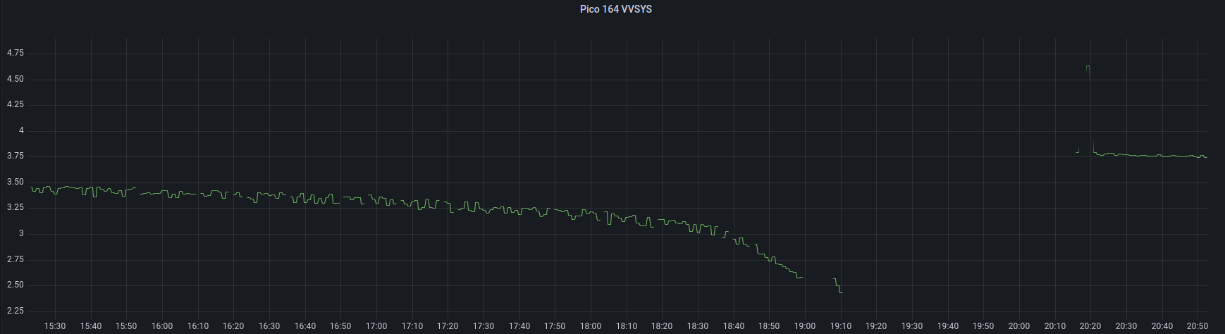
While ideally the answer to this problem is to improve our data gathering process, this isn’t always going to be possible. The good news is that Grafana has our back.
If we go to the ‘Edit’ function for a panel (found in the drop-down that opens up by clicking on the panel name) and scroll down the list of options we come to the ‘Connect null values’ setting under the ‘Graph styles’ heading.
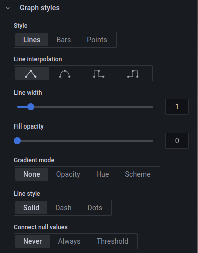
Here we have three options. The first, ‘Never’ means that if we get any null values (no data has been recorded) then we will see gaps in the corresponding places in the graph (like the one above).
If we select ‘Always’ Grafana will automatically connect any two adjacent data points so that the graph looks a little more normal.
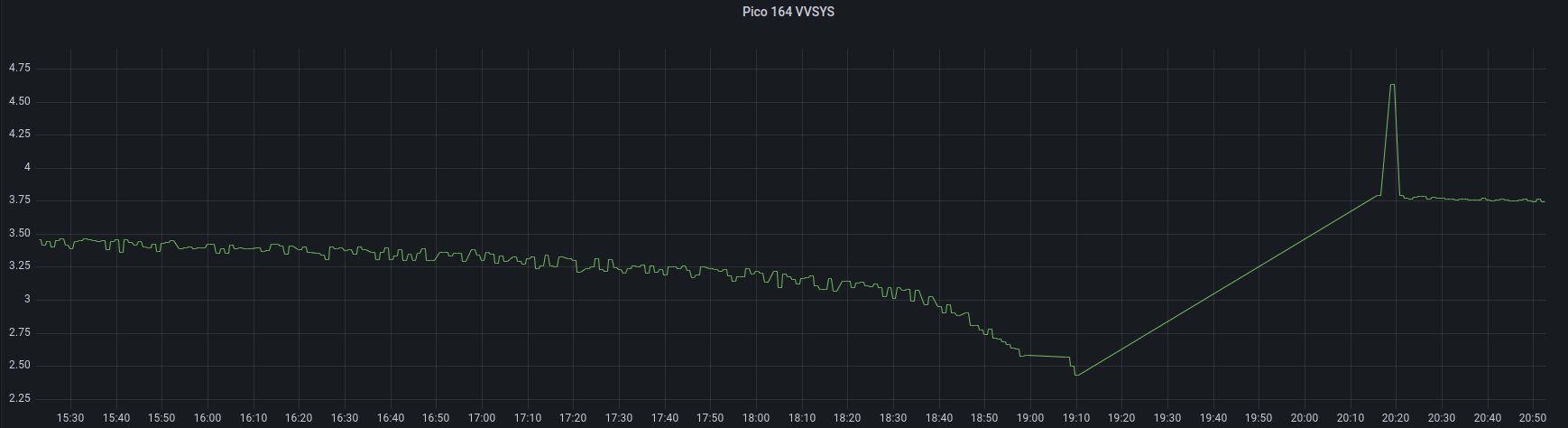
Of course, that might not be what we are wanting as the graph above shows two fairly separate battery discharge curves and in between time, there was no voltage from the battery and therefore no data collected. So if we were being picky we would like to see our small gaps filled in, but the larger ones left in place.
Grafana <hold my beer>.
So the following graph is the result of selecting ‘Threshold’ for ‘Connect null values’. In this setting adjacent data points will be connected if they fall under the threshold set. If there are no values (nulls) for the length of time in the threshold, then there will be a gap in the graph like below.
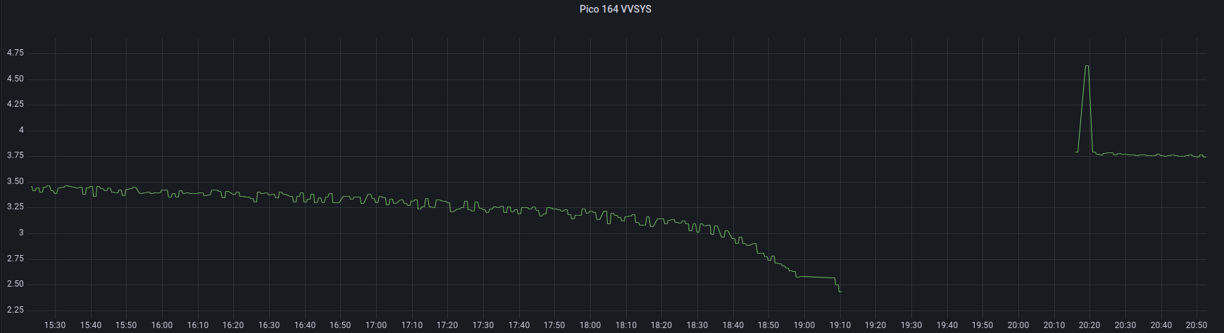
Well played Grafana. Well played.
Exporting Data from a Grafana Graph
While using Grafana is a wonderful experience and it’s hard to imagine improving on the options and nuance that we can gather from a Grafana panel, occasionally we will find ourselves in a situation where we want to export some of the data that we can see in a graph.
Nothing could be simpler.
Just click on the name of the graph panel which will open up a drop-down menu. Select ‘Inspect’ and then ‘Data’.
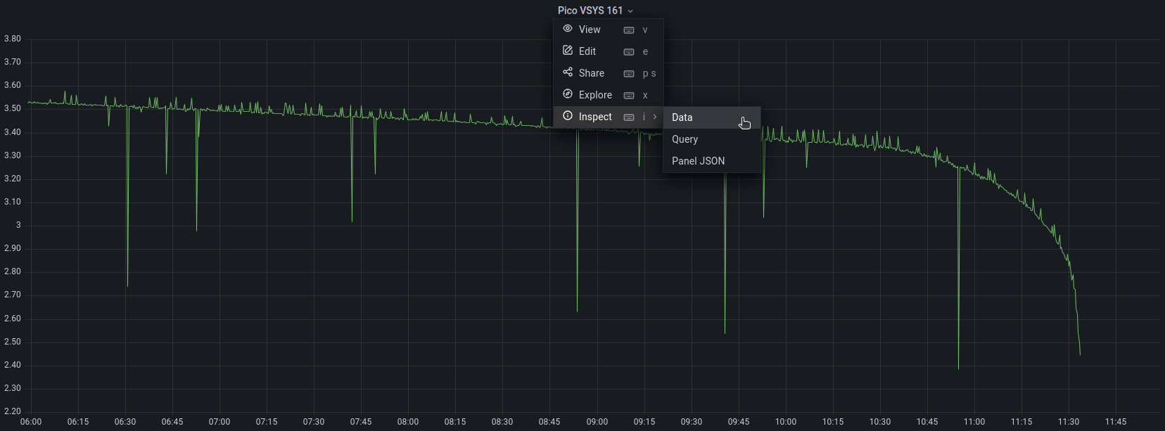
This will then show a page where we can check out the data at our own leisure and it even provides an option for downloading the data as a CSV file.
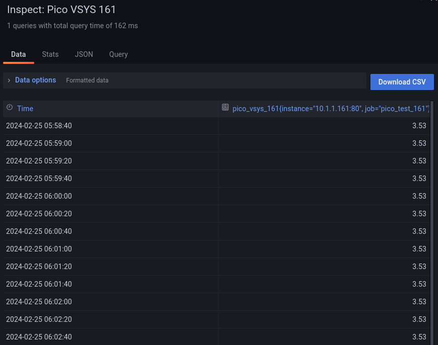
Nice!
Linux Concepts
What is Linux?
In it’s simplest form, the answer to the question “What is Linux?” is that it’s a computer operating system. As such it is the software that forms a base that allows applications that run on that operating system to run.
In the strictest way of speaking, the term ‘Linux’ refers to the Linux kernel. That is to say the central core of the operating system, but the term is often used to describe the set of programs, tools, and services that are bundled together with the Linux kernel to provide a fully functional operating system.
An operating system is software that manages computer hardware and software resources for computer applications. For example Microsoft Windows could be the operating system that will allow the browser application Firefox to run on our desktop computer.
Linux is a computer operating system that is can be distributed as free and open-source software. The defining component of Linux is the Linux kernel, an operating system kernel first released on 5 October 1991 by Linus Torvalds.
Linux was originally developed as a free operating system for Intel x86-based personal computers. It has since been made available to a huge range of computer hardware platforms and is a leading operating system on servers, mainframe computers and supercomputers. Linux also runs on embedded systems, which are devices whose operating system is typically built into the firmware and is highly tailored to the system; this includes mobile phones, tablet computers, network routers, facility automation controls, televisions and video game consoles. Android, the most widely used operating system for tablets and smart-phones, is built on top of the Linux kernel.

The development of Linux is one of the most prominent examples of free and open-source software collaboration. Typically, Linux is packaged in a form known as a Linux distribution, for both desktop and server use. Popular mainstream Linux distributions include Debian, Ubuntu and the commercial Red Hat Enterprise Linux. Linux distributions include the Linux kernel, supporting utilities and libraries and usually a large amount of application software to carry out the distribution’s intended use.
A distribution intended to run as a server may omit all graphical desktop environments from the standard install, and instead include other software to set up and operate a solution stack such as LAMP (Linux, Apache, MySQL and PHP). Because Linux is freely re-distributable, anyone may create a distribution for any intended use.
Linux is not an operating system that people will typically use on their desktop computers at home and as such, regular computer users can find the barrier to entry for using Linux high. This is made easier through the use of Graphical User Interfaces that are included with many Linux distributions, but these graphical overlays are something of a shim to the underlying workings of the computer. There is a greater degree of control and flexibility to be gained by working with Linux at what is called the ‘Command Line’ (or CLI), and the booming field of educational computer elements such as the Raspberry Pi have provided access to a new world of learning opportunities at this more fundamental level.
Linux Directory Structure
To a new user of Linux, the file structure may feel like something at best arcane and in some cases arbitrary. Of course this isn’t entirely the case and in spite of some distribution specific differences, there is a fairly well laid out hierarchy of directories and files with a good reason for being where they are.
We are frequently comfortable with the concept of navigating this structure using a graphical interface similar to that shown below, but to operate effectively at the command line we need to have a working knowledge of what goes where.
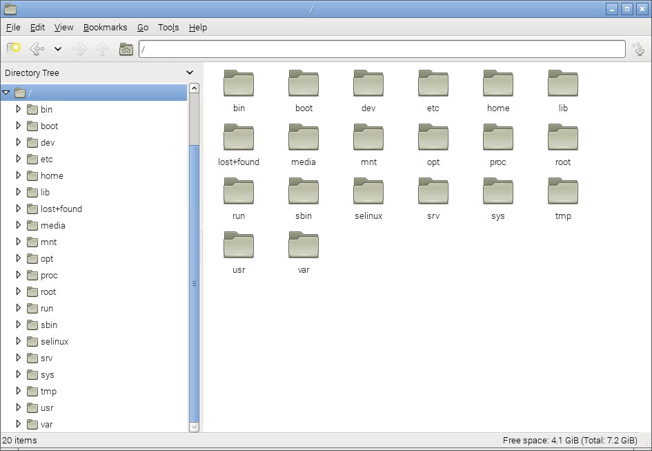
The directories we are going to describe form a hierarchy similar to the following;
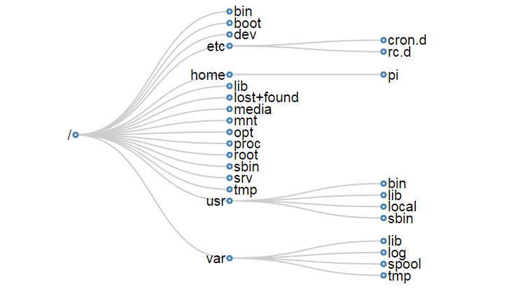
For a concise description of the directory functions check out the cheat sheet. Alternatively their function and descriptions are as follows;
/
The / or ‘root’ directory contains all other files and directories. It is important to note that this is not the root users home directory (although it used to be many years ago). The root user’s home directory is /root. Only the root user has write privileges for this directory.
/bin
The /bin directory contains common essential binary executables / commands for use by all users. For example: the commands cd, cp, ls and ping. These are commands that may be used by both the system administrator and by users, but which are required when no other filesystems are mounted.
/boot
The /boot directory contains the files needed to successfully start the computer during the boot process. As such the /boot directory contains information that is accessed before the Linux kernel begins running the programs and process that allow the operating system to function.
/dev
The /dev directory holds device files that represent physical devices attached to the computer such as hard drives, sound devices and communication ports as well as ‘logical’ devices such as a random number generator and /dev/null which will essentially discard any information sent to it. This directory holds a range of files that strongly reinforces the Linux precept that Everything is a file.
/etc
The /etc directory contains configuration files that control the operation of programs. It also contains scripts used to startup and shutdown individual programs.
/etc/cron.d
The /etc/cron.d, /etc/cron.hourly, /etc/cron.daily, /etc/cron.weekly, /etc/cron.monthly directories contain scripts which are executed on a regular schedule by the crontab process.
/etc/rc?.d
The /rc0.d, /rc1.d, /rc2.d, /rc3.d, /rc4.d, /rc5.d, /rc6.d, /rcS.d directories contain the files required to control system services and configure the mode of operation (runlevel) for the computer.
/home
Because Linux is an operating system that is a ‘multi-user’ environment, each user requires a space to store information specific to them. This is done via the /home directory. For example, the user ‘pi’ would have /home/pi as their home directory.
/lib
The /lib directory contains shared library files that supports the executable files located under /bin and /sbin. It also holds the kernel modules (drivers) responsible for giving Linux a great deal of versatility to add or remove functionality as needs dictate.
/lost+found
The /lost+found directory will contain potentially recoverable data that might be produced if the file system undergoes an improper shut-down due to a crash or power failure. The data recovered is unlikely to be complete or undamaged, but in some circumstances it may hold useful information or pointers to the reason for the improper shut-down.
/media
The /media directory is used as a directory to temporarily mount removable devices (for example, /media/cdrom or /media/cdrecorder). This is a relatively new development for Linux and comes as a result of a degree of historical confusion over where was best to mount these types of devices (/cdrom, /mnt or /mnt/cdrom for example).
/mnt
The /mnt directory is used as a generic mount point for filesystems or devices. Recent use of the directory is directing it towards it being used as a temporary mount point for system administrators, but there is a degree of historical variation that has resulted in different distributions doing things different ways (for example, Debian allocates /floppy and /cdrom as mount points while Redhat places them in /mnt/floppy and /mnt/cdrom respectively).
/opt
The /opt directory is used for the installation of third party or additional optional software that is not part of the default installation. Any applications installed in this area should be installed in such a way that it conforms to a reasonable structure and should not install files outside the /opt directory.
/proc
The /proc directory holds files that contain information about running processes and system resources. It can be described as a pseudo filesystem in the sense that it contains runtime system information, but not ‘real’ files in the normal sense of the word. For example the /proc/cpuinfo file which contains information about the computers cpus is listed as 0 bytes in length and yet if it is listed it will produce a description of the cpus in use.
/root
The /root directory is the home directory of the System Administrator, or the ‘root’ user. This could be viewed as slightly confusing as all other users home directories are in the /home directory and there is already a directory referred to as the ‘root’ directory (/). However, rest assured that there is good reason for doing this (sometimes the /home directory could be mounted on a separate file system that has to be accessed as a remote share).
/sbin
The /sbin directory is similar to the /bin directory in the sense that it holds binary executables / commands, but the ones in /sbin are essential to the working of the operating system and are identified as being those that the system administrator would use in maintaining the system. Examples of these commands are fdisk, shutdown, ifconfig and modprobe.
/srv
The /srv directory is set aside to provide a location for storing data for specific services. The rationale behind using this directory is that processes or services which require a single location and directory hierarchy for data and scripts can have a consistent placement across systems.
/tmp
The /tmp directory is set aside as a location where programs or users that require a temporary location for storing files or data can do so on the understanding that when a system is rebooted or shut down, this location is cleared and the contents deleted.
/usr
The /usr directory serves as a directory where user programs and data are stored and shared. This potential wide range of files and information can make the /usr directory fairly large and complex, so it contains several subdirectories that mirror those in the root (/) directory to make organisation more consistent.
/usr/bin
The /usr/bin directory contains binary executable files for users. The distinction between /bin and /usr/bin is that /bin contains the essential commands required to operate the system even if no other file system is mounted and /usr/bin contains the programs that users will require to do normal tasks. For example; awk, curl, php, python. If you can’t find a user binary under /bin, look under /usr/bin.
/usr/lib
The /usr/lib directory is the equivalent of the /lib directory in that it contains shared library files that supports the executable files for users located under /usr/bin and /usr/sbin.
/usr/local
The /usr/local directory contains users programs that are installed locally from source code. It is placed here specifically to avoid being inadvertently overwritten if the system software is upgraded.
/usr/sbin
The /usr/sbin directory contains non-essential binary executables which are used by the system administrator. For example cron and useradd. If you can’t locate a system binary in /usr/sbin, try /sbin.
/var
The /var directory contains variable data files. These are files that are expected to grow under normal circumstances For example, log files or spool directories for printer queues.
/var/lib
The /var/lib directory holds dynamic state information that programs typically modify while they run. This can be used to preserve the state of an application between reboots or even to share state information between different instances of the same application.
/var/log
The /var/log directory holds log files from a range of programs and services. Files in /var/log can often grow quite large and care should be taken to ensure that the size of the directory is managed appropriately. This can be done with the logrotate program.
/var/spool
The /var/spool directory contains what are called ‘spool’ files that contain data stored for later processing. For example, printers which will queue print jobs in a spool file for eventual printing and then deletion when the resource (the printer) becomes available.
/var/tmp
The /var/tmp directory is a temporary store for data that needs to be held between reboots (unlike /tmp).
Everything is a file in Linux
A phrase that will often come up in Linux conversation is that;
Everything is a file
For someone new to Linux this sounds like some sort of ‘in joke’ that is designed to scare off the unwary and it can sometimes act as a barrier to a deeper understanding of the philosophy behind the approach taken in developing Linux.
The explanation behind the statement is that Linux is designed to be a system built of a group of interacting parts and the way that those parts can work together is to communicate using a common method. That method is to use a file as a common building block and the data in a file as the communications mechanism.
The trick to understanding what ‘Everything is a file’ means, is to broaden our understanding of what a file can be.
Traditional Files
The traditional concept of a file is an object with a specific name in a specific location with a particular content. For example, we might have a file named foo.txt which is in the directory /home/pi/ and it could contain a couple of lines of text similar to the following;
Directories
As unusual as it sounds a directory is also a file. The special aspect of a directory is that is is a file which contains a list of information about which files (and / or subdirectories) it contains. So when we want to list the contents of a directory using the ls command what is actually happening is that the operating system is getting the appropriate information from the file that represents the directory.
System Information
However, files can also be conduits of information. The /proc/ directory contains files that represent system and process information. If we want to determine information about the type of CPU that the computer is using, the file cpuinfo in the /proc/ directory can list it. By running the command `cat /proc/cpuinfo’ we can list a wealth of information about our CPU (the following is a subset of that information by the way);
Now that might not mean a lot to us at this stage, but if we were writing a program that needed a particular type of CPU in order to run successfully it could check this file to ensure that it could operate successfully. There are a wide range of files in the /proc/ directory that represent a great deal of information about how our system is operating.
Devices
When we use different devices in a Linux operating system these are also represented as a file. In the /dev/ directory we have files that represent a range of physical devices that are part of our computer. In larger computer systems with multiple disks they could be represented as /dev/sda1 and /dev/sda2, so that when we wanted to perform an action such as formatting a drive we would use the command mkfs on the /dev/sda1 file.
The /dev/ directory also holds some curious files that are used as tools for generating or managing data. For example /dev/random is an interface to the kernels random number device. /dev/zero represents a file that will constantly stream zeros (while this might sound weird, imagine a situation where you want to write over an area of disk with data to erase it). The most well known of these unusual files is probably /dev/null. This will act as a ‘null device’ that will essentially discard any information sent to it.
File Editing
Working in Linux is an exercise in understanding the concepts that Linux uses as its foundations such as ‘Everything is a file’ and the use of wildcards, pipes and the directory structure.
While working at the command line there will very quickly come the realisation that there is a need to know how to edit a file. Linux being what it is, there are many ways that files can be edited.
An outstanding illustration of this is via the excellent cartoon work of the xkcd comic strip (Buy his stuff, it’s awesome!).

For a taste of the possible options available Wikipedia has got our back. Inevitably where there is choice there are preferences and where there are preferences there is bias. Everyone will have a preference towards a particular editor and don’t let a particular bias influence you to go down a particular direction without considering your options. Speaking from personal experience I was encouraged to use ‘vi’ as it represented the preference of the group I was in, but because I was a late starter to the command line I struggled for the longest time to try and become familiar with it. I know I should have tried harder, but I failed. For a while I wandered in the editor wilderness trying desperately to cling to the GUI where I could use ‘gedit’ or ‘geany’ and then one day I was introduced to ‘nano’.
This has become my preference and I am therefore biased towards it. Don’t take my word for it. Try alternatives. I’ll describe ‘nano’ below, but take that as a possible path and realise that whatever editor works for you will be the right one. The trick is simply to find one that works for you.
The nano Editor
The nano editor can be started from the command line using just the command and the /path/name of the file.
If the file requires administrator permissions it can be executed with ‘sudo`.
When it opens it presents us with a working space and part of the file and some common shortcuts for use at the bottom of the console;
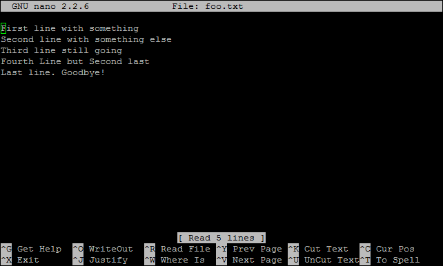
It includes some simple syntax highlighting for common file formats;
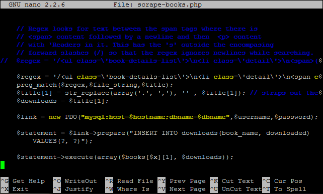
This can be improved if desired (cue Google).
There is a swag of shortcuts to make editing easier, but the simple ones are as follows;
- CTRL-x - Exit the editor. If we are in the middle of editing a file we will be asked if we want to save our work
- CTRL-r - Read a file into our current working file. This enables us to add text from another file while working from within a new file.
- CTRL-k - Cut text.
- CTRL-u - Uncut (or Paste) text.
- CTRL-o - Save file name and continue working.
- CTRL-t - Check the spelling of our text.
- CTRL-w - Search the text.
- CTRL-a - Go to the beginning of the current working line.
- CTRL-e - Go to the end of the current working line.
- CTRL-g - Get help with nano.
Linux Commands
Executing Commands in Linux
A command is an instruction given by a user telling the computer to carry out an action. This could be to run a single program or a group of linked programs. Commands are typically initiated by typing them in at the command line (in a terminal) and then pressing the ENTER key, which passes them to the shell.
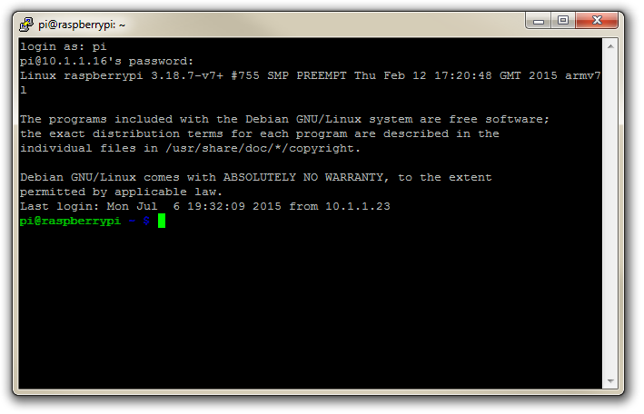
A terminal refers to a wrapper program which runs a shell. This used to mean a physical device consisting of little more than a monitor and keyboard. As Unix/Linux systems advanced the terminal concept was abstracted into software. Now we have programs such as LXTerminal (on the Raspberry Pi) which will launch a window in a Graphical User Interface (GUI) which will run a shell into which you can enter commands. Alternatively we can dispense with the GUI all together and simply start at the command line when we boot up.
The shell is a program which actually processes commands and returns output. Every Linux operating system has at least one shell, and most have several. The default shell on most Linux systems is bash.
The Commands
Commands on Linux operating systems are either built-in or external commands. Built-in commands are part of the shell. External commands are either executables (programs written in a programming language and then compiled into an executable binary) or shell scripts.
A command consists of a command name usually followed by one or more sequences of characters that include options and/or arguments. Each of these strings is separated by white space. The general syntax for commands is;
commandname [options] [arguments]
The square brackets indicate that the enclosed items are optional. Commands typically have a few options and utilise arguments. However, there are some commands that do not accept arguments, and a few with no options.
As an example we can run the ls command with no options or arguments as follows;
The ls command will list the contents of a directory and in this case the command and the output would be expected to look something like the following;
Options
An option (also referred to as a switch or a flag) is a single-letter code, or sometimes a single word or set of words, that modifies the behaviour of a command. When multiple single-letter options are used, all the letters are placed adjacent to each other (not separated by spaces) and can be in any order. The set of options must usually be preceded by a single hyphen, again with no intervening space.
So again using ls if we introduce the option -l we can show the total files in the directory and subdirectories, the names of the files in the current directory, their permissions, the number of subdirectories in directories listed, the size of the file, and the date of last modification.
The command we execute therefore looks like this;
And so the command (with the -l option) and the output would look like the following;
26
drwxr-xr-x 2 pi pi 4096 Feb 20 08:07 Desktop
drwxrwxr-x 2 pi pi 4096 Jan 27 08:34 python_games
Here we can see quite a radical change in the formatting and content of the returned information.
Arguments
An argument (also called a command line argument) is a file name or other data that is provided to a command in order for the command to use it as an input.
Using ls again we can specify that we wish to list the contents of the python_games directory (which we could see when we ran ls) by using the name of the directory as the argument as follows;
The command (with the python_games argument) and the output would look like the following (actually I removed quite a few files to make it a bit more readable);
Putting it all together
And as our final example we can combine our command (ls) with both an option (-l) and an argument (python_games) as follows;
Hopefully by this stage, the output shouldn’t come as too much surprise, although again I have pruned some of the files for readabilities sake;
1800
-rw-rw-r-- 1 pi pi 9731 Jan 27 08:34 4row_arrow.png
-rw-rw-r-- 1 pi pi 7463 Jan 27 08:34 4row_black.png
-rw-rw-r-- 1 pi pi 8666 Jan 27 08:34 4row_board.png
-rw-rw-r-- 1 pi pi 18933 Jan 27 08:34 4row_computerwinner.png
-rw-rw-r-- 1 pi pi 25412 Jan 27 08:34 4row_humanwinner.png
-rw-rw-r-- 1 pi pi 8562 Jan 27 08:34 4row_red.png
-rw-rw-r-- 1 pi pi 14661 Jan 27 08:34 tetrisc.mid
-rw-rw-r-- 1 pi pi 15759 Jan 27 08:34 tetrominoforidiots.py
-rw-rw-r-- 1 pi pi 18679 Jan 27 08:34 tetromino.py
-rw-rw-r-- 1 pi pi 9771 Jan 27 08:34 Tree_Short.png
-rw-rw-r-- 1 pi pi 11546 Jan 27 08:34 Tree_Tall.png
-rw-rw-r-- 1 pi pi 10378 Jan 27 08:34 Tree_Ugly.png
-rw-rw-r-- 1 pi pi 8443 Jan 27 08:34 Wall_Block_Tall.png
-rw-rw-r-- 1 pi pi 6011 Jan 27 08:34 Wood_Block_Tall.png
-rw-rw-r-- 1 pi pi 8118 Jan 27 08:34 wormy.py
apt-get
The apt-get command is a program, that is used with Debian based Linux distributions to install, remove or upgrade software packages. It’s a vital tool for installing and managing software and should be used on a regular basis to ensure that software is up to date and security patching requirements are met.
There are a plethora of uses for apt-get, but we will consider the basics that will allow us to get by. These will include;
- Updating the database of available applications (
apt-get update) - Upgrading the applications on the system (
apt-get upgrade) - Installing an application (
apt-get install *package-name*) - Un-installing an application (
apt-get remove *package-name*)
The apt-get command
The apt part of apt-get stands for ‘advanced packaging tool’. The program is a process for managing software packages installed on Linux machines, or more specifically Debian based Linux machines (Since those based on ‘redhat’ typically use their rpm (red hat package management (or more lately the recursively named ‘rpm package management’) system). As the Raspberry Pi OS is based on Debian, so the examples we will be using are based on apt-get.
APT simplifies the process of managing software on Unix-like computer systems by automating the retrieval, configuration and installation of software packages. This was historically a process best described as ‘dependency hell’ where the requirements for different packages could mean a manual installation of a simple software application could lead a user into a sink-hole of despair.
In common apt-get usage we will be prefixing the command with sudo to give ourselves the appropriate permissions;
apt-get update
This will resynchronize our local list of packages files, updating information about new and recently changed packages. If an apt-get upgrade (see below) is planned, an apt-get update should always be performed first.
Once the command is executed, the computer will delve into the internet to source the lists of current packages and download them so that we will see a list of software sources similar to the following appear;
[490 B]
Get:2 http://archive.raspberrypi.org wheezy Release.gpg [473 B]
Hit http://raspberrypi.collabora.com wheezy Release
Get:3 http://mirrordirector.raspbian.org wheezy Release [14.4 kB]
Get:4 http://archive.raspberrypi.org wheezy Release [17.6 kB]
Hit http://raspberrypi.collabora.com wheezy/rpi armhf Packages
Get:5 http://mirrordirector.raspbian.org wheezy/main armhf Packages [6,904 kB]
Get:6 http://archive.raspberrypi.org wheezy/main armhf Packages [130 kB]
Ign http://raspberrypi.collabora.com wheezy/rpi Translation-en
Ign http://mirrordirector.raspbian.org wheezy/contrib Translation-en
Ign http://mirrordirector.raspbian.org wheezy/main Translation-en
Ign http://mirrordirector.raspbian.org wheezy/non-free Translation-en
Ign http://mirrordirector.raspbian.org wheezy/rpi Translation-en
Fetched 7,140 kB in 35s (200 kB/s)
Reading package lists... Done
apt-get upgrade
The apt-get upgrade command will install the newest versions of all packages currently installed on the system. If a package is currently installed and a new version is available, it will be retrieved and upgraded. Any new versions of current packages that cannot be upgraded without changing the install status of another package will be left as they are.
As mentioned above, an apt-get update should always be performed first so that apt-get upgrade knows which new versions of packages are available.
Once the command is executed, the computer will consider its installed applications against the databases list of the most up to date packages and it will prompt us with a message that will let us know how many packages are available for upgrade, how much data will need to be downloaded and what impact this will have on our local storage. At this point we get to decide whether or not we want to continue;
6 upgraded, 0 newly installed, 0 to remove and 0 not upgraded.
Need to get 10.7 MB of archives.
After this operation, 556 kB disk space will be freed.
Do you want to continue [Y/n]?
Once we say yes (‘Y’) the upgrade kicks off and we will see a list of the packages as they are downloaded unpacked and installed (what follows is an edited example);
continue [Y/n]? y
Get:1 http://archive.raspberrypi.org/debian/wheezy/main libsdl1.2debian
armhf 1.2.15-5+rpi1 [205 kB]
Get:2 http://archive.raspberrypi.org/debian/wheezy/main raspi-config all
20150131-5 [13.3 kB]
Get:3 http://mirrordirector.raspbian.org/raspbian/ wheezy/main libsqlite3-0
armhf 3.7.13-1+deb7u2 [414 kB]
Fetched 10.7 MB in 31s (343 kB/s)
Preconfiguring packages ...
(Reading database ... 80703 files and directories currently installed.)
Preparing to replace cups-common 1.5.3-5+deb7u5
(using .../cups-common_1.5.3-5+deb7u6_all.deb) ...
Unpacking replacement cups-common ...
Preparing to replace cups-bsd 1.5.3-5+deb7u5
(using .../cups-bsd_1.5.3-5+deb7u6_armhf.deb) ...
Unpacking replacement cups-bsd ...
Preparing to replace php5-gd 5.4.39-0+deb7u2
(using .../php5-gd_5.4.41-0+deb7u1_armhf.deb) ...
Unpacking replacement php5-gd ...
Processing triggers for man-db ...
Setting up libssl1.0.0:armhf (1.0.1e-2+rvt+deb7u17) ...
Setting up libsqlite3-0:armhf (3.7.13-1+deb7u2) ...
Setting up cups-common (1.5.3-5+deb7u6) ...
Setting up cups-client (1.5.3-5+deb7u6) ...
There can often be alerts as the process identifies different issues that it thinks the system might strike (different aliases, runtime levels or missing fully qualified domain names). This is not necessarily a sign of problems so much as an indication that the process had to take certain configurations into account when upgrading and these are worth noting. Whenever there is any doubt about what has occurred, Google will be your friend :-).
apt-get install
The apt-get install command installs or upgrades one (or more) packages. All additional (dependency) packages required will also be retrieved and installed.
If we want to install multiple packages we can simply list each package separated by a space after the command as follows;
apt-get remove
The apt-get remove command removes one (or more) packages.
cd
The cd command is used to move around in the directory structure of the file system (change directory). It is one of the fundamental commands for navigating the Linux directory structure.
cd [options] directory : Used to change the current directory.
For example, when we first log into the Raspberry Pi as the ‘pi’ user we will find ourselves in the /home/pi directory. If we wanted to change into the /home directory (go up a level) we could use the command;
Take some time to get familiar with the concept of moving around the directory structure from the command line as it is an important skill to establish early in Linux.
The cd command
The cd command will be one of the first commands that someone starting with Linux will use. It is used to move around in the directory structure of the file system (hence cd = change directory). It only has two options and these are seldom used. The arguments consist of pointing to the directory that we want to go to and these can be absolute or relative paths.
The cd command can be used without options or arguments. In this case it returns us to our home directory as specified in the /etc/passwd file.
If we cd into any random directory (try cd /var) we can then run cd by itself;
… and in the case of a vanilla installation of the Raspberry Pi OS, we will change to the /home/pi directory;
cd /var
pi@raspberrypi /var $ cd
pi@raspberrypi ~ $ pwd
/home/pi
In the example above, we changed to /var and then ran the cd command by itself and then we ran the pwd command which showed us that the present working directory is /home/pi. This is the Raspberry Pi OS default home directory for the pi user.
Options
As mentioned, there are only two options available to use with the cd command. This is -P which instructs cd to use the physical directory structure instead of following symbolic links and the -L option which forces symbolic links to be followed.
For those beginning Linux, there is little likelihood of using either of these two options in the immediate future and I suggest that you use your valuable memory to remember other Linux stuff.
Arguments
As mentioned earlier, the default argument (if none is included) is to return to the users home directory as specified in the /etc/passwd file.
When specifying a directory we can do this by absolute or relative addressing. So if we started in the /home/pi directory, we could go the /home directory by executing;
… or using relative addressing and we can use the .. symbols to designate the parent directory;
Once in the /home directory, we can change into the /home/pi/Desktop directory using relative addressing as follows;
We can also use the - argument to navigate to the previous directory we were in.
Examples
Change into the root (/) directory;
Test yourself
- Having just changed from the
/home/pidirectory to the/homedirectory, what are the five variations of using thecdcommand that will take the pi user to the/home/pidirectory - Starting in the
/home/pidirectory and using only relative addressing, usecdto change into the/vardirectory.
ifconfig
The ifconfig command can be used to view the configuration of, or to configure a network interface. Networking is a fundamental function of modern computers. ifconfig allows us to configure the network interfaces to allow that connection.
-
ifconfig[arguments] [interface]
or
-
ifconfig[arguments] interface [options]
Used with no ‘interface’ declared ifconfig will display information about all the operational network interfaces. For example running;
… produces something similar to the following on a simple Raspberry Pi.
76:12:45:56:47:53
UP BROADCAST MULTICAST MTU:1500 Metric:1
RX packets:0 errors:0 dropped:0 overruns:0 frame:0
TX packets:0 errors:0 dropped:0 overruns:0 carrier:0
collisions:0 txqueuelen:1000
RX bytes:0 (0.0 B) TX bytes:0 (0.0 B)
lo Link encap:Local Loopback
inet addr:127.0.0.1 Mask:255.0.0.0
UP LOOPBACK RUNNING MTU:65536 Metric:1
RX packets:0 errors:0 dropped:0 overruns:0 frame:0
TX packets:0 errors:0 dropped:0 overruns:0 carrier:0
collisions:0 txqueuelen:0
RX bytes:0 (0.0 B) TX bytes:0 (0.0 B)
wlan0 Link encap:Ethernet HWaddr 09:87:65:54:43:32
inet addr:10.1.1.8 Bcast:10.1.1.255 Mask:255.255.255.0
UP BROADCAST RUNNING MULTICAST MTU:1500 Metric:1
RX packets:3978 errors:0 dropped:898 overruns:0 frame:0
TX packets:347 errors:0 dropped:0 overruns:0 carrier:0
collisions:0 txqueuelen:1000
RX bytes:859773 (839.6 KiB) TX bytes:39625 (38.6 KiB)
The output above is broken into three sections; eth0, lo and wlan0.
-
eth0is the first Ethernet interface and in our case represents the RJ45 network port on the Raspberry Pi (in this specific case on a B+ model). If we had more than one Ethernet interface, they would be namedeth1,eth2, etc. -
lois the loopback interface. This is a special network interface that the system uses to communicate with itself. You can notice that it has the IP address 127.0.0.1 assigned to it. This is described as designating the ‘localhost’. -
wlan0is the name of the first wireless network interface on the computer. This reflects a wireless USB adapter (if installed). Any additional wireless interfaces would be namedwlan1,wlan2, etc.
The ifconfig command
The ifconfig command is used to read and manage a servers network interface configuration (hence ifconfig = interface configuration).
We can use the ifconfig command to display the current network configuration information, set up an ip address, netmask or broadcast address on an network interface, create an alias for network interface, set up hardware addresses and enable or disable network interfaces.
To view the details of a specific interface we can specify that interface as an argument;
Which will produce something similar to the following;
(8.4 MiB) TX bytes:879127 (858.5 KiB)
The configuration details being displayed above can be interpreted as follows;
-
Link encap:Ethernet- This tells us that the interface is an Ethernet related device. -
HWaddr b8:27:eb:2c:bc:62- This is the hardware address or Media Access Control (MAC) address which is unique to each Ethernet card. Kind of like a serial number. -
inet addr:10.1.1.8- indicates the interfaces IP address. -
Bcast:10.1.1.255- denotes the interfaces broadcast address -
Mask:255.255.255.0- is the network mask for that interface. -
UP- Indicates that the kernel modules for the Ethernet interface have been loaded. -
BROADCAST- Tells us that the Ethernet device supports broadcasting (used to obtain IP address via DHCP). -
RUNNING- Lets us know that the interface is ready to accept data. -
MULTICAST- Indicates that the Ethernet interface supports multicasting. -
MTU:1500- Short for for Maximum Transmission Unit is the size of each packet received by the Ethernet card. -
Metric:1- The value for the Metric of an interface decides the priority of the device (to designate which of more than one devices should be used for routing packets). -
RX packets:119833 errors:0 dropped:0 overruns:0 frame:0andTX packets:8279 errors:0 dropped:0 overruns:0 carrier:0- Show the total number of packets received and transmitted with their respective errors, number of dropped packets and overruns respectively. -
collisions:0- Shows the number of packets which are colliding while traversing the network. -
txqueuelen:1000- Tells us the length of the transmit queue of the device. -
RX bytes:8895891 (8.4 MiB)andTX bytes:879127 (858.5 KiB)- Indicates the total amount of data that has passed through the Ethernet interface in transmit and receive.
Options
The main option that would be used with ifconfig is -a which will will display all of the interfaces on the interfaces available (ones that are ‘up’ (active) and ‘down’ (shut down). The default use of the ifconfig command without any arguments or options will display only the active interfaces.
Arguments
We can disable an interface (turn it down) by specifying the interface name and using the suffix ‘down’ as follows;
Or we can make it active (bring it up) by specifying the interface name and using the suffix ‘up’ as follows;
To assign a IP address to a specific interface we can specify the interface name and use the IP address as the suffix;
To add a netmask to a a specific interface we can specify the interface name and use the netmask argument followed by the netmask value;
To assign an IP address and a netmask at the same time we can combine the arguments into the same command;
Test yourself
- List all the network interfaces on your server.
- Why might it be a bad idea to turn down a network interface while working on a server remotely?
- Display the information about a specific interface, turn it down, display the information about it again then turn it up. What differences do you see?
mv
The mv command is used to rename and move files or directories. It is one of the basic Linux commands that allow for management of files from the command line.
-
mv[options] source destination : Move and/or rename files and directories
For example: to rename the file foo.txt and to call it foo-2.txt we would enter the following;
This makes the assumption that we are in the same directory as the file foo.txt, but even if we weren’t we could explicitly name the file with the directory structure and thereby not just rename the file, but move it somewhere different;
To move the file without renaming it we would simply omit the new name at the destination as so;
The mv command
The mv command is used to move or rename files and directories (mv is an abbreviated form of the word move). This is a similar command to the cp (copy) command but it does not create a duplicate of the files it is acting on.
If we want to move multiple files, we can put them on the same line separated by spaces.
The normal set of wildcards and addressing options are available to make the process more flexible and extensible.
Options
While there are a few options available for the mv command the one most commonly ones used would be -u and -i.
-
uThis updates moved files by only moving the file when the source file is newer than the destination file or when the destination file does not exist. -
iInitiates an interactive mode where we are prompted for confirmation whenever the move would overwrite an existing target.
Examples
To move all the files from directory1 to directory2 (directory2 must initially exist);
To rename a directory from directory1 to directory2 (directory2 must not already exist);
To move the files foo.txt and bar.txt to the directory foobar;
To move all the ‘txt’ files from the users home directory to a directory called backup but to only do so if the file being moved is newer than the destination file;
Test yourself
- How can we move a file to a new location when that act might overwrite an already existing file?
- What characters cannot be used when naming directories or files?
rm
The rm command is used to remove file or directories. This is a basic Linux file management command that should be understood by all Linux users.
-
rm[options] file : Delete files or directories
For example if we want to remove the file foo.txt we would use the command as follows;
The rm command
The rm command is used to remove (hence rm = remove) files. Any act that involves deleting files should be treated with a degree of caution and the rm command falls into the ‘treat with caution’ category. This is especially true if using wildcards or complex relative addressing.
It will not remove directories by default although it can be directed to do so via the -r option (covered later). The command will return an error message if a file doesn’t exist or if the user doesn’t have the appropriate permissions to delete it. Files which are located in write-protected directories can not be removed, even if those files are not write-protected (they are protected by the directory).
If a file to be deleted is a symbolic link, the link will be removed, but the file or directory to which that link refers will not be deleted.
Options
There are a small number of options available for use with rm. The following would be the most common;
-
-rallows us to recursivly remove directories and their contents -
-fallows us to force the removal of files irrespective of write-protected status -
-itells thermcommend to interactivly prompt us for confirmation of every deletion
So the following will delete the foobar directory and all its contents;
To delete all the txt files in the current directory irrespective of their write-protect status (and without prompting us to tell us that it’s happening);
To take a nice careful approach and to have a prompt for the removal of each file we can use the -i option. The following example will look for each txt file and ask us if we want to delete it;
The output will look something like the following;
We can’t use the -f and -i options simultaneously. Whichever was the last one in the command takes affect.
The rm command supports the -- (two consecutive dashes) parameter which acts as a delimiter that indicates the end of any options. This is used when the name of a file or directory begins with a dash. For example, the following removes a directory named -directory1;
Arguments
The normal set of wildcards and addressing options are available to make the process of finding the right files more flexible and extensible.
To remove more than one file we can simply separate them with a space as follows;
Test yourself
- Will the
-foption successfully delete a write protected file in a write protected directory? Justify your answer. - What are the implications of running the following command;
sudo
The sudo command allows a user to execute a command as the ‘superuser’ (or as another user). It is a vital tool for system administration and management.
-
sudo[options] [command] : Execute a command as the superuser
For example, if we want to update and upgrade our software packages, we will need to do so as the super user. All we need to do is prefix the command apt-get with sudo as follows;
One of the best illustrations of this is via the excellent cartoon work of the xkcd comic strip (Buy his stuff, it’s awesome!).

The sudo command
The sudo command is shorthand for ‘superuser do’.
When we use sudo an authorised user is determined by the contents of the file /etc/sudoers.
As an example of usage we should check out the file /etc/sudoers. If we use the cat command to list the file like so;
We get the following response;
That’s correct, the ‘pi’ user does not have permissions to view the file
Let’s confirm that with ls;
Which will result in the following;
1 root root 696 May 7 10:39 /etc/sudoers
It would appear that only the root user can read the file!
So let’s use sudo to cat](#cat) the file as follows;
That will result in the following output;
There’s a lot of information in the file, but there, right at the bottom is the line that determines the privileges for the ‘pi’ user;
We can break down what each section means;
pi
pi ALL=(ALL) NOPASSWD: ALL
The pi portion is the user that this particular rule will apply to.
ALL
pi ALL=(ALL) NOPASSWD: ALL
The first ALL portion tells us that the rule applies to all hosts.
ALL
pi ALL=(ALL) NOPASSWD: ALL
The second ALL tells us that the user ‘pi’ can run commands as all users and all groups.
NOPASSWD
pi ALL=(ALL) NOPASSWD: ALL
The NOPASSWD tells us that the user ‘pi’ won’t be asked for their password when executing a command with sudo.
All
pi ALL=(ALL) NOPASSWD: ALL`
The last ALL tells us that the rules on the line apply to all commands.
Under normal situations the use of sudo would require a user to be authorised and then enter their password. By default the Raspberry Pi OS operating system has the ‘pi’ user configured in the /etc/sudoers file to avoid entering the password every time.
If your curious about what privileges (if any) a user has, we can execute sudo with the -l option to list them;
This will result in output that looks similar to the following;
for pi on this host:
env_reset, mail_badpass,
secure_path=/usr/local/sbin\:/usr/local/bin\:/usr/sbin\:/usr/bin\:/sbin\:/bin
User pi may run the following commands on this host:
(ALL : ALL) ALL
(ALL) NOPASSWD: ALL
The ‘sudoers’ file
As mentioned above, the file that determines permissions for users is /etc/sudoers. DO NOT EDIT THIS BY HAND. Use the visudo command to edit. Of course you will be required to run the command using sudo;
sudo vs su
There is a degree of confusion about the roles of the sudo command vs the su command. While both can be used to gain root privileges, the su command actually switches the user to another user, while sudo only runs the specified command with different privileges. While there will be a degree of debate about their use, it is widely agreed that for simple on-off elevation, sudo is ideal.
Test yourself
- Write an entry for the
sudoersfile that provides sudo privileges to a user for only thecatcommand. - Under what circumstances can you edit the
sudoersfile with a standard text editor.
tar
The tar command is designed to facilitate the creation of an archive of files by combining a range of files and directories into a single file and providing the ability to extract these files again. While tar does not include compression as part of its base function, it is available via an option. tar is a useful program for archiving data and as such forms an important command for good maintenance of files and systems.
-
tar[options] archivename [file(s)] : archive or extract files
tar is renowned as a command that has a plethora of options and flexibility. So much so that it can appear slightly arcane and (dare I say it) ‘over-flexible’. This has been well illustrated in the excellent cartoon work of the xkcd comic strip (Buy his stuff, it’s awesome!).

However, just because it has a lot of options does not mean that it needs to be difficult to use for a standard set of tasks and at its most basic is the creation of an archive of files as follows;
Here we are creating an archive in a file called foobar.tar of the files foo.txt and bar.txt.
The options used allow us to;
-
c: create a new archive -
v: verbosely list files which are processed. -
f: specify the following name as the archive file name
The output of the command is the echoing of the files that are placed in the archive;
The additional result is the creation of the file containing our archive foobar.tar.
To carry the example through to its logical conclusion we would want to extract the files from the archive as follows;
The options used allow us to;
-
x: extract an archive -
v: verbosely list files which are processed. -
f: specify the following name as the archive file name
The output of the command is the echoing of the files that are extracted from the archive;
The tar command
tape archive, or tar for short, is a command for converting files and directories into a single data file. While originally written for reading and writing from sequential devices such as tape drives, it is nowadays used more commonly as a file archive tool. In this sense it can be considered similar to archiving tools such as WinZip or 7zip. The resulting file created as a result of using the tar command is commonly called a ‘tarball’.
Note that tar does not provide any compression, so in order to reduce the size of a tarball we need to use an external compression utility such as gzip. While this is the most common, any other compression type can be used. These switches are the equivalent of piping the created archive through gzip.
One advantage to using tar over other archiving tools such as zip is that tar is designed to preserve Unix filesystem features such as user and group permissions, access and modification dates, and directory structures.
Another advantage to using tar for compressed archives is the fact that any compression is applied to the tarball in its entirety, rather than individual files within the archive as is the case with zip files. This allows for more efficient compression as the process can take advantage of data redundancy across multiple files.
Options
-
c: Create a new tar archive. -
x: Extract a tar archive. -
f: Work on a file. -
z: Use Gzip compression or decompression when creating or extracting. -
t: List the contents of a tar archive.
The tar program does not compress the files, but it can incorporate the gzip compression via the -z option as follows;
If we want to lit the contents of a tarball without un-archiving it we can use the -t option as follows;
When using tar to distribute files to others it is considered good etiquette to have the tarball extract into a directory of the same name as the tar file itself. This saves the recipient from having a mess of files on their hands when they extract the archive. Think of it the same way as giving your friends a set of books. They would much rather you hand them a box than dump a pile of loose books on the floor.
For example, if you wish to distribute the files in the foodir directory then we would create a tarball from the directory containing these files, rather than the files themselves:
Remember that tar operates recursively by default, so we don’t need to specify all of the files below this directory ourselves.
Test yourself
- Do you need to include the
zoption when decompressing atararchive? - Enter a valid tar command on the first try. No Googling. You have 10 seconds.
wget
The wget command (or perhaps a better description is ‘utility’) is a program designed to make downloading files from the Internet easy using the command line. It supports the HTTP, HTTPS and FTP protocols and is designed to be robust to accomplish its job even on a network connection that is slow or unstable. It is similar in function to curl for retrieving files, but there are some key differences between the two, with the main one for wget being that it is capable of downloading files recursively (where resources are linked from web pages).
-
wget[options] [URL] : download or upload files from the web non-interactivly.
In it’s simplest example of use it is only necessary to provide the URL of the file that is required and the download will begin;
The program will then connect to the remote server, confirm the file details and start downloading the file;
As the downloading process proceeds a simple text animation advises of the progress with an indication of the amount downloaded and the rate
Once complete the successful download will be reported accompanied by some statistics of the transfer;
The file is downloaded into the current working directory.
The wget command
wget is a utility that exists slightly out of the scope of a pure command in the sense that it is an Open Source program that has been complied to work on a range of operating systems. The name is a derivation of web get where the function of the program is to ‘get’ files from the world wide web.
It does this via support for the HTTP, HTTPS and FTP protocols such that if you could paste a URL in a browser and have it subsequently download a file, the same file could be downloaded from the command line using wget. wget is not the only file downloading utility that is commonly used in Linux. curl is also widely used for similar functions. However both programs have different strengths and in the case of wget that strength is in support of recursive downloading where an entire web site could be downloaded while maintaining its directory structure and links. There are other differences as well, but this would be the major one.
There is a large range of options that can be used to ensure that downloads are configured correctly. We will examine a few of the more basic examples below and after that we will check out the recursive function of wget.
-
--limit-rate: limit the download speed / download rate. -
-O: download and store with a different file name -
-b: download in the background -
-i: download multiple files / URLs -
--ftp-userand--ftp-password: FTP download using wget with username and password authentication
Rate limit the bandwidth
There will be times when we will be somewhere that the bandwidth is limited or we want to prioritise the bandwidth in some way. We can restrict the download speed with the option --limit-rate as follows;
Here we’ve limited the download speed to 20 kilo bytes per second. The amount may be expressed in bytes, kilobytes with the k suffix, or megabytes with the m suffix.
Rename the downloaded file
If we try to download a file with the same name into the working directory it will be saved with an incrementing numerical suffix (i.e. .1, .2 etc). However, we can give the file a different name when downloaded using the -O option (that’s a capital ‘o’ by the way). For example to save the file with the name alpha.zip we would do the following;
Download in the background
Because it may take some considerable time to download a file we can tell the process to run in the background which will release the terminal to carry on working. This is accomplished with the -b option as follows;
While the download continues, the progress that would normally be echoed to the screen is passed to the file wget-log that will be in the working directory. We can check this file to determine progress as necessary.
Download multiple files
While we can download multiple files by simply including them one after the other in the command as follows;
While that is good, it can start to get a little confusing if a large number of URL’s are included. To make things easier, we can create a text file with the URL’s/names of the files we want to download and then we specify the file with the -i option.
For example, if we have a file named files.txt in the current working directory that has the following contents;
Then we can run the command…
… and it will work through each file and download it.
Download files that require a username and password
The examples shown thus far have been able to be downloaded without providing any form of authentication (no user / password). However this will be a requirement for some downloads. To include a username and password in the command we include the --ftp-user and --ftp-password options. For example if we needed to use the username ‘adam’ and the password ‘1234’ we would form or command as follows;
You may be thinking to yourself “Is this secure?”. To which the answer should probably be “No”. It is one step above anonymous access, but not a lot more. This is not a method by which things that should remain private should be secured, but it does provide a method of restricting anonymous access.
Download files recursively
One of the main features of wget is it’s ability to download a large complex directory structure that exists on many levels. The best example of this would be the structure of files and directories that exist to make up a web site. While there is a wide range of options that can be passed to make the process work properly in a wide variety of situations, it is still possible to use a fairly generic set to get us going.
For example, to download the contents of the web site at dnoob.runkite.com we can execute the following command;
The options used here do the following;
-
-e robots=off: the execute option allows us to run a separate command and in this case it’s the commandrobots=offwhich tells the web site that we are visiting that it should ignore the fact that we’re running a command that is acting like a robot and to allow us to download the files. -
-r: the recursive option enables recursive downloading. -
-np: the no-parent option makes sure that a recursive retrieval only works on pages that are below the specified directory. -
-c: the continue option ensures that any partially downloaded file continues from the place it left off. -
-nc: the no-clobber option ensures that duplicate files are not overridden
Once entered the program will display a running listing of the progress and a summary telling us how many file and the time taken at the end. The end result is a directory called dnoob.runkite.com in the working directory that has the entire website including all the linked pages and files in it. If we examine the directory structure it will look a little like the following;
Using wget for recursive downloading should be used appropriately. It would be considered poor manners to pillage a web site for anything other than good reason. When in doubt contact the person responsible for a site or a repository just to make sure there isn’t a simpler way that you might be able to accomplish your task if it’s something ‘weird’.
Test yourself
- Craft a
wgetcommand that downloads a file to a different name, limiting the download rate to 10 kilobytes per second and which operates in the background. - Once question 1 above is carried out, where do we find the output of the downloads progress?
Directory Structure Cheat Sheet
-
/: The ‘root’ directory which contains all other files and directories -
/bin: Common commands / programs, shared by all users -
/boot: Contains the files needed to successfully start the computer during the boot process -
/dev: Holds device files that represent physical and ‘logical’ devices -
/etc: Contains configuration files that control the operation of programs -
/etc/cron.d: One of the directories that allow programs to be run on a regular schedule -
/etc/rc?.d: Directories containing files that control the mode of operation of a computer -
/home: A directory that holds subdirectories for each user to store user specific files -
/lib: Contains shared library files and kernel modules -
/lost+found: Will hold recoverable data in the event of an an improper shut-down -
/media: Used to temporarily mount removable devices -
/mnt: A mount point for filesystems or temporary mount point for system administrators -
/opt: Contains third party or additional software that is not part of the default installation -
/proc: Holds files that contain information about running processes and system resources -
/root: The home directory of the System Administrator, or the ‘root’ user -
/sbin: Contains binary executables / commands used by the system administrator -
/srv: Provides a consistent location for storing data for specific services -
/tmp: A temporary location for storing files or data -
/usr: Is the directory where user programs and data are stored and shared -
/usr/bin: Contains binary executable files for users -
/usr/lib: Holds shared library files to support executables in/usr/binand/usr/sbin -
/usr/local: Contains users programs that are installed locally from source code -
/usr/sbin: The directory for non-essential system administration binary executables -
/var: Holds variable data files which are expected to grow under normal circumstances -
/var/lib: Contains dynamic state information that programs modify while they run -
/var/log: Stores log files from a range of programs and services -
/var/spool: Contains files that are held (spooled) for later processing -
/var/tmp: A temporary store for data that needs to be held between reboots (unlike/tmp)